Science blog of a physics theorist Feed

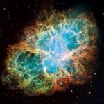
On April 8th, 2024, a small strip of North America will witness a total solar eclipse. Total solar eclipses are amazing, life-changing experiences; I hope you have a chance to experience one, as I did.

Everyone else from Central America to northern Canada will see a partial solar eclipse. What good is a partial solar eclipse?

Astonishingly, the best thing about a partial solar eclipse seems to have essentially disappeared from public knowledge. We’ve got three weeks to change that, and I hope you’ll help me — especially the science journalists and science teachers among you.

The best thing about a partial solar eclipse is that you can measure the Moon’s true diameter, armed with only a map, a straight-edge, and a leafy tree or a card with a pinhole in it. No telescope, no eclipse glasses, no equipment that costs real money or is hard to obtain. You’ll get an answer that’s good within 10-20 percent, with no effort at all. And in the process you can teach kids about shadows, about simple geometry (no trigonometry needed), about the Earth, Moon, and Sun, and about how scientists figure things out.

About a week later, you can measure the Moon’s distance from Earth, too. All you need for that is a coin, a ruler, and drawings of similar triangles.

In this post, I’ll explain

• First, the two easy steps necessary to measure the size of the Moon;
• Second, evidence that this actually works;
• Third, the reasons why it works;
• Fourth, a brief comment (and a link to an older, longer post about it) showing how to measure the Moon’s distance once you know its size

The Amazingly Easy Way to Measure the Size of the Moon

1. Before the eclipse, find a map that shows your location and the “totality strip” where the eclipse is total. On that map, measure the smallest linear distance (not the driving distance!) between you and the edge of the strip. Call that distance L.
   
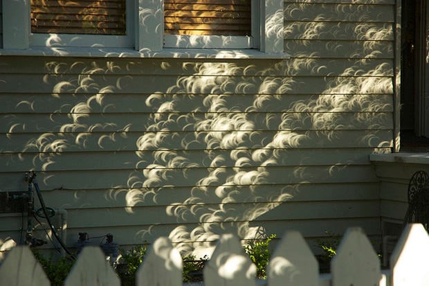
2. Next, right at the maximum of the eclipse, when the Moon’s silhouette blocks as much of the Sun as it can from your location, determine the fraction of the Sun’s diameter that remains visible, measured at the thickest part of the Sun’s shape. (You can see the shape of the eclipsed Sun where it is projected onto the ground or a piece of paper, after the sunlight has passed through leaves, or through a colander, or through a grid of your own fingers, or through any other little hole through which light can pass.) Call that fraction F.

Then the diameter of the Moon D is roughly equal to L divided by F:

That’s all there is to it!

This estimate should be accurate to within 10-20% (as long as you’re not too close to the Earth’s poles or too close to the totality strip; we can talk about why later.) Any child over ten can carry this out with a little help.

Click here to see an example of how this works

From Boston, here’s how I can measure L, using Google Maps and an eclipse map showing the location of the totality strip:

From Boston to the totality strip is about 145 miles.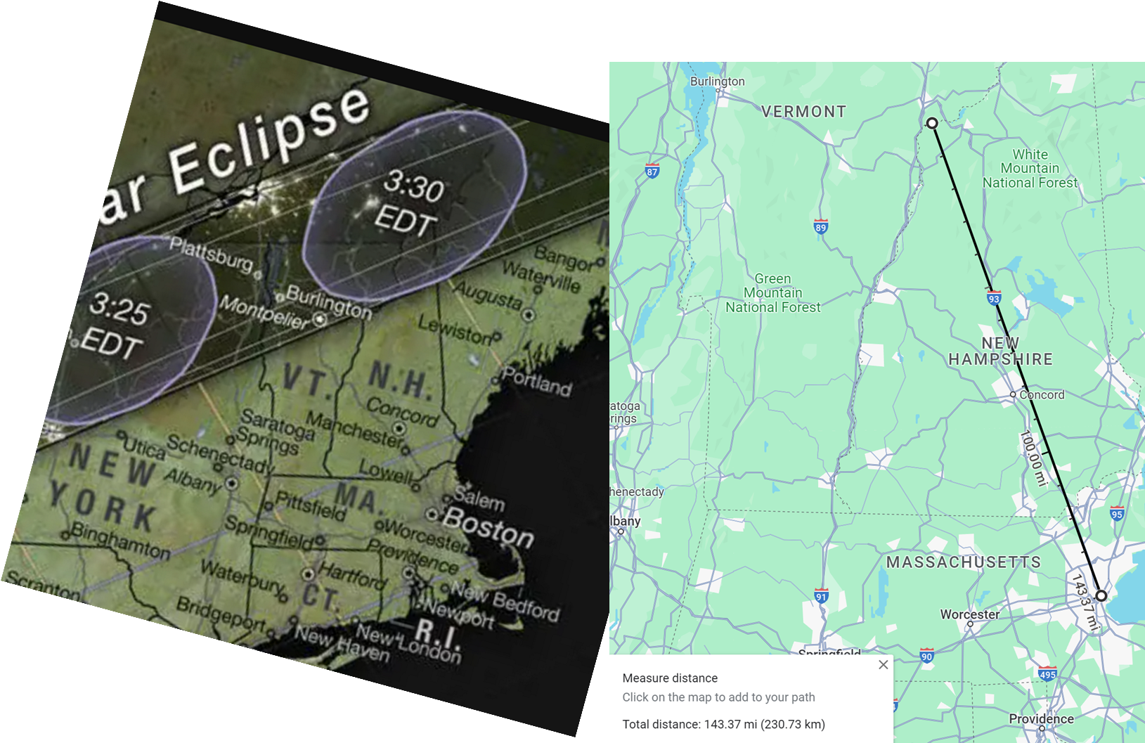

Meanwhile timeanddate.com predicts that in Boston at mid-eclipse the Sun will appear as shown below: a fraction of around 6 to 8% of the Sun will be unblocked. (We’re so close to the totality strip that measuring F is quite difficult to do accurately, so our estimate of the Moon’s size will be more uncertain than for people further away.)

The fraction of the Sun’s diameter that will be visible at mid-eclipse in Boston is less than 10%; the full diameter of the Sun is shown in orange. Prediction from timeanddate.com .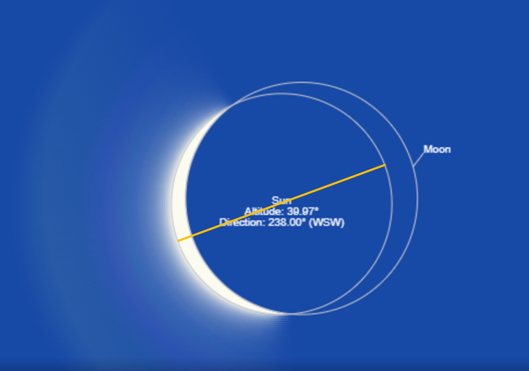

That will give us (if we take F=7% as a best guess) an estimate of the Moon’s size

• D = L / F = 143 miles / 0.07 = 2050 miles .

(If we let F range from 6% to 8%, this estimate really ranges between 1900 and 2200 miles.) The Moon’s true diameter is about 2160 miles, so this is wonderfully successful, given its ease.

Is this too good to be true? Let’s see.

Some Basic Evidence

Here’s a map from NASA (via Wikipedia) showing where the eclipse is total and partial. Let’s call the region of totality the “totality strip”, and the regions where the eclipse is partial the “northern partiality zone” and the “southern partiality zone.”

Figure 1: As with all total eclipses, the one on April 8th will have a narrow totality strip (dark blue) where the eclipse is total, surrounded by two large “partiality zones” (light blue) in which the eclipse will be partial. Eclipse Predictions by Fred Espenak, NASA’s GSFC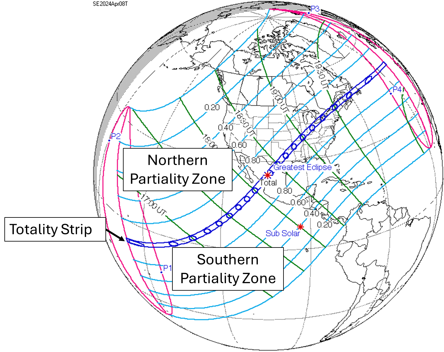

Now here’s the same map with the Moon, correctly sized, superposed on the two partiality zones. You see that indeed the width of each partiality zone is roughly the size of the Moon — slightly larger, but much less than twice as large. [Because the eclipse is north of the equator, the northern partiality zone is closer to the north pole, and the Earth’s curvature causes it to be somewhat larger than the southern partiality zone. This is discussed in an aside later in this post.]

Figure 2: Each partiality strip is a little wider than the diameter of the Moon, for reasons explained later.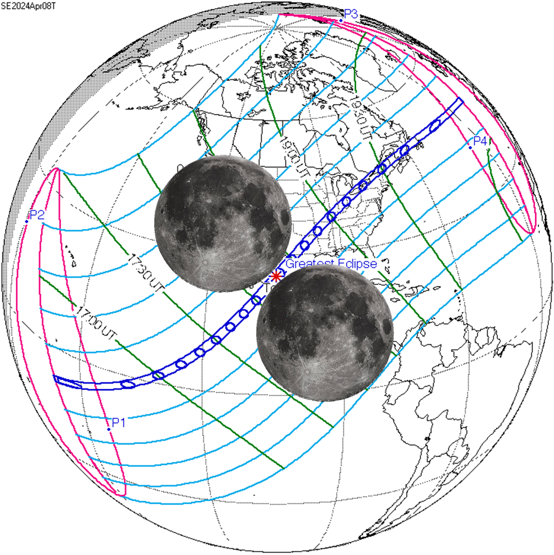

Let’s say you’re in one of the partiality zones, and let’s call its width W. If you’re right near the outer edge of that zone, then L is approximately W. That’s also where the eclipse barely happens — the Moon just clips the edge of the Sun — and so, since the Sun’s diameter is hardly blocked at all, F is close to 1. Your estimate will then be

• D = L / F = W / 1 = W,

which is in accord with Figure 2.

Suppose instead that you are halfway between the totality strip and the outer edge of your zone (measured on a line perpendicular to the totality strip.) Then L = W/2. But also the Moon will block half the Sun’s diameter, leaving half of it unblocked: F = 1/2. That means that you will estimate, again,

• D = L/F = (W/2) / (1/2) = W.

More generally, if your distance from the totality strip is L, and L is a fraction P of the width W of the partiality zone, i.e.

• L = P W ,

then the fraction F of the Sun’s diameter that will be unblocked at mid-eclipse will also be approximately P. Therefore, no matter where you are in the zone,

• D = L / F = (P W) / P = W ,

so your estimate of the Moon’s diameter will always come out more or less right.

(That said, if you’re very close to the totality strip, F will be hard to measure precisely, so your estimate may be very uncertain; and if you’re close to the poles, W will be significantly larger than D, so your estimate will be poor. Fortunately, that won’t be true for most of us.)

What’s behind this clever trick? Here’s the reasoning.

Why Does This Work?

What’s great about this trick is that it’s not hard to understand, though it does take a few steps. [I’m not sure I yet have the best pedagogical strategy for laying out those steps; suggestions welcome.]

Why the Partiality Zones are as Wide as the Moon

First, we need to understand why the width of each partiality zone is roughly the same as the width of the Moon — why D and W are almost the same, as long as we are far from the Earth’s poles. It all has to do with shadows — moon shadows, of both types.

You may have noticed (kids often do) that there are often two types of shadows visible when you’re at home and lit by a single central light. If a thumbtack lit by a small light bulb is close to a wall, it casts a shadow that is crisp and about the same size as the tack. But as you move the tack away from the wall, the shadow becomes fuzzier. If you look closely, you’ll see that the inner dark part of the shadow (the “umbra”) is shrinking, while there’s an outer part (the “penumbra”), quite hard to see, that is growing.

Eventually, when the tack is far enough away, the inner dark part will become almost a dot. At that point, the outer dim shadow — you may only barely see it — has a diameter about twice the diameter of the tack. See Figure 3.

Figure 3: How a shadow of a tack changes as it moves away from the wall. (Left) The shadow is crisp and the same size as the tack. (Center) The dark umbra is narrower than the tack, while the dim penumbra is wider than the tack. (Right) As the dark umbra becomes very narrow, the penumbra becomes twice the width of the tack (as indicated by the two tack-sized disks). Credit: the author.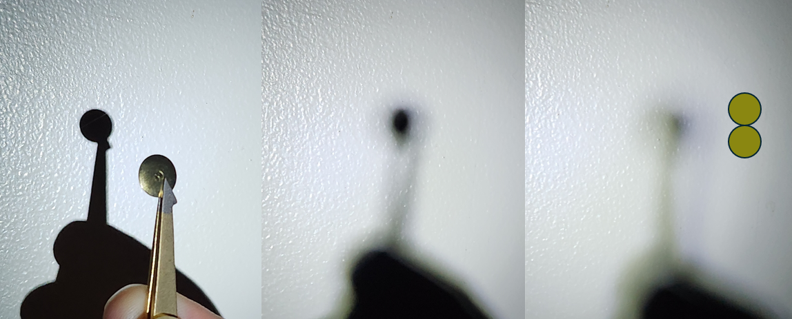

For the solar eclipse, it’s the same idea, except that instead of bulb, tack and wall, we have Sun, Moon and Earth.

There’s simple geometry behind this shadow-play; I’ve drawn it vertically in the figure below, so that you can see it no matter how narrow your screen. Let’s assume that the Sun is much further away from Earth than the Moon is (a fact that you can also verify during daytime, either a week after the eclipse or a week before.) I’ve drawn four lines, two of them red, two of them black; watch where they go.

Figure 4: The Sun is totally eclipsed in the little gap between the black lines; it is partially eclipsed between the red and black lines. Not to scale.

Inside the black lines, the Moon totally blocks the Sun; both the left edge and right edge of the Sun in the figure are blocked. Inside the red lines, the Moon partially blocks the Sun. And so, at the moment shown, the little space between the two black lines is where the eclipse is total; that’s a location within the totality strip. Meanwhile, the distance between each red line and the nearest black line is the width W of one of the partiality zones.

For maximum simplicity, I’ve drawn this where the Sun, Moon and Earth are perfectly lined up, so that the total eclipse is occuring where the Earth’s surface is nearest the Sun and Moon. That makes both partiality zones the same size. In the aside below, I’ll show you what happens if this isn’t the case. But let’s not get distracted by that yet.

The important thing is that because the Sun is so much further than the Moon, the red and black lines from the left edge of the Sun are almost parallel. Where they meet the Moon, they are separated by the Moon’s diameter — that is, by the distance D. But the distance between two parallel lines is constant, so the distance between two nearly parallel lines changes very slowly. This means they are still a distance D apart when they reach the Earth.

On top of this, the two black lines almost meet; the totality strip is very narrow. Taken together, these facts imply that W, the width of the region on Earth’s surface between a red line and the closest black line, is roughly the same size as D!

As noted in an aside below, the Earth’s curvature tends to make the partiality zones a bit larger than the Moon’s diameter, while for an eclipse nearing a pole of the Earth, the partiality zone closest to the pole will be larger than the other partiality zone. But these are details; they don’t change the basic story.

Click here for an brief discussion of why W and D aren’t quite the same

As noted, W isn’t quite D. Even with the eclipse centered on the Earth as in Figure 5, W is larger than D because the Earth’s surface is a sphere. (This is somewhat compensated for by measuring L to the edge of the totality zone rather than its center or opposite edge.)

The width W of the partiality zone is wider than the diameter D of the Moon because of the Earth’s shape.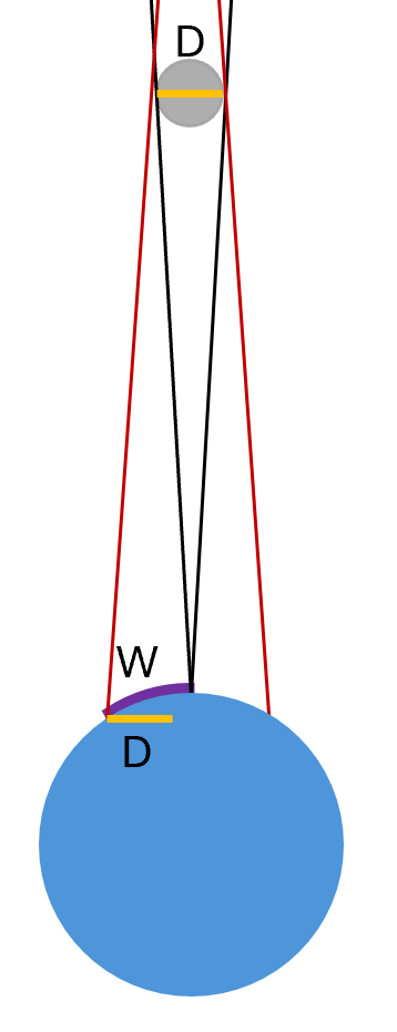

Second, if the eclipse is far from the equator, the partiality zone nearer to a pole of the Earth will be larger than the other.

If the location of totality is offset from the line connecting Moon and Sun, then the totality zone on the side of the offset will be larger than the other, and than D, due to the Earth’s curvature.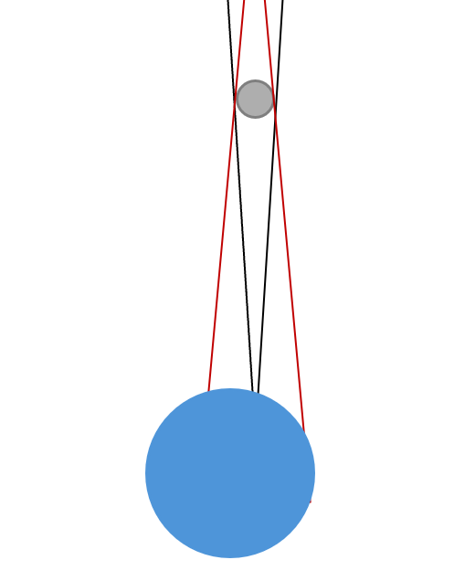

In short, this is not a method designed to get a precise or accurate measurement of the Moon’s diameter. But it’s perfectly fine if one’s aim is merely to get a rough idea of how nature works, which is often more than enough for scientists, as well as for everyone else. There is an opportunity here to talk to students about the nature of approximations, when and why it’s okay to use them, and how to improve upon them.

Why the Unblocked Fraction of the Sun’s Diameter Plays the Key Role

Second, we have to understand why the unblocked fraction F of the Sun’s diameter is roughly the same as what we called P (the distance L to the totality strip divided by the width of the partiality zone W.) This is illustrated in Figure 5, where again I’ve drawn four lines on each image, but now all four begin from the location at which we are observing the eclipse, and they indicate where the Moon and Sun appear to us.

Figure 5: What one sees in the partiality zone between the red and black dots; the orange and grey lines show the location and width on the sky of the Sun and Moon.(Far Left) In the totality zone, F=P=0. (Far Right) Near the edge of the partiality zone, F and P are close to 1. (Near Left and Right) Throughout the partiality zone, F=P, as shown for P=1/6 and 1/2. Not to scale.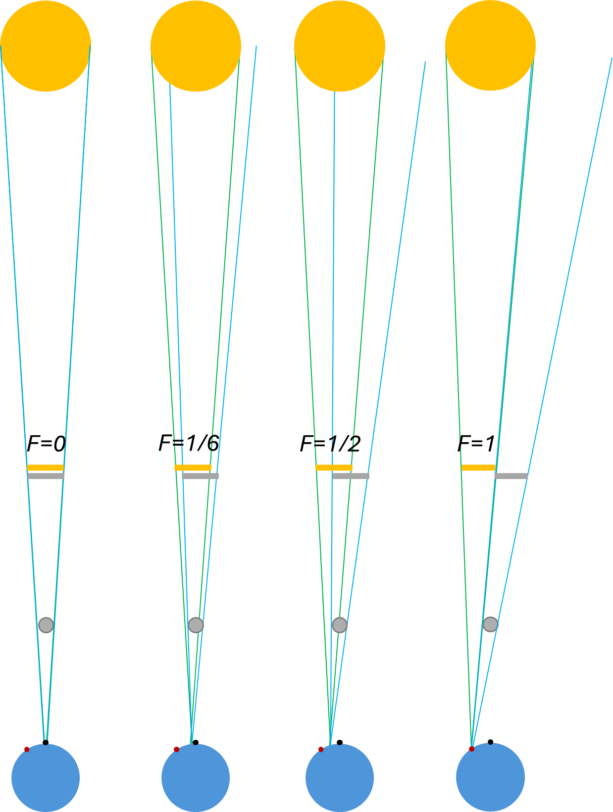

In each image in Figure 5, the totality strip is indicated by the black dot, and the edge of a partiality zone by the red dot. The Sun’s disk in the sky is spanned by the green lines, and its apparent width in the sky is shown by the orange line; the Moon’s disk is spanned by the blue lines, and its apparent width is shown by the grey line.

In the far left image, the observer is in the totality strip, so P=0; the Moon blocks the Sun completely, so the grey line aligns with the orange line and F=0. At far right, the observer is at the outer edge of the partiality zone, so P is almost 1; the grey line almost misses the orange line completely, so almost all the Sun’s diameter remains unblocked and F is almost 1. In between are shown intermediate situations where F and P are both 1/6 or both 1/2. The closer the observer gets to the totality strip, making P smaller, the less of the Sun is unblocked, making F smaller by the same amount.

Bonus: Measure the Distance to the Moon in Daylight

I’ve explained how this works in this older post. For today, here’s a quick summary.

Within a week after the eclipse, the Moon will reach first quarter, which means that the Moon will rise around noon. In the afternoon, then, you can see it in the East. Then you can have one person hold a penny, and another person move until the penny perfectly eclipses the Moon; a third person can measure the distance s between the person’s eyes and the penny. Then, measuring the diameter d of the penny, we can use similar triangles to convince ourselves that the distance S to the Moon, divided by the diameter of the Moon D, is the same as the distance from observer to penny divided by the diameter of the penny:

• S/D = s/d

and so

• S = (s/d) D

Since we measured D during the eclipse, we now know S also.

By the way, in another old post, I showed that we can also confirm that our original assumption, that the Sun is much, much further than the Moon, is correct. At first quarter — i.e. one quarter of the way through the Moon’s monthly cycle — one can verify two things at once, by eye:

• the Moon is half lit
• the Moon is 90 degrees away from the Sun in the sky

These two things can only both be true if the Sun is much further than the Moon.

Spread the Word

So you see, it’s not only easy to measure the Moon’s size during an eclipse, it’s relatively easy to explain how and why the method works. To do so requires a range of logical reasoning tools, some drawings of lines and triangles, and a little experimentation with shadows, but no actual math. (I’m sure it can be done better than I did it here.) On top of that, the measurement can be carried out in daylight, while most children are in school. I think it’s a great opportunity for science education — a chance for a meaningful fraction of the 600 million people in North America to experience scientific reasoning for themselves, and to observe how it leads to consistent, reliable knowledge.

Already I’ve had a few people ask me for clarification of a key point in the book, having to do with a certain type of unusual “standing wave.” It’s so central to the story that I’ve decided to address it right away.

The point that there are two quite different types of standing waves; the familiar ones you may know from musical instruments or from physics class, and less familiar ones that play a key role in the book. You can jump right to my new webpage comparing these two types of standing waves, or you can read the post below, which provides more context.

Note: Going forward, you’ll see a lot of posts and new webpages like this one. One of the great things about 21st century books is that they aren’t contained within their covers. I’ve always planned to continue the book into this website, allowing me to expand here upon key issues that I knew would will raise questions from readers. So even though the book in printed form is done and published, it will continue to live and grow on this website.

The Stationary Electron as a Standing Wave

In the book’s chapter 17, I suggest a sort of mental image of a stationary electron. In particular, electrons should be visualized as waves, not as little dots, and a stationary electron is a standing wave — a wave that vibrates in place. [I focus on a stationary electron because it’s the best context in which to understand an electron’s “rest mass” (see chapters 5 and 8.)]

If you know something about standing waves already, perhaps from music classes or from a first-year physics class, this statement is potentially confusing. An electron could be stationary out in the middle of nowhere, light-years from the nearest star. But the standing waves of music and physics classes are never found in the middle of nowhere; they are always found inside or upon objects of finite size, perhaps upon a guitar string, inside a room or in the Sun. So how could a free-floating, isolated electron out in the open be a standing wave?

This mismatch is naturally puzzling, and indeed it has already raised questions among listeners of my recent podcast appearances. [Here’s the conversation on Sean Carroll’s podcast, and here are the first half and second half of the conversation with Daniel Whiteson on his podcast.]

The point, which I didn’t have time to address in the podcasts and which is discussed in the book only in examples (see chapter 20.2), is that there is a type of standing wave that is not covered in first-year physics classes, and that appears in no human musical instruments that I’m aquainted with. Unlike familiar standing waves, it needs no walls.

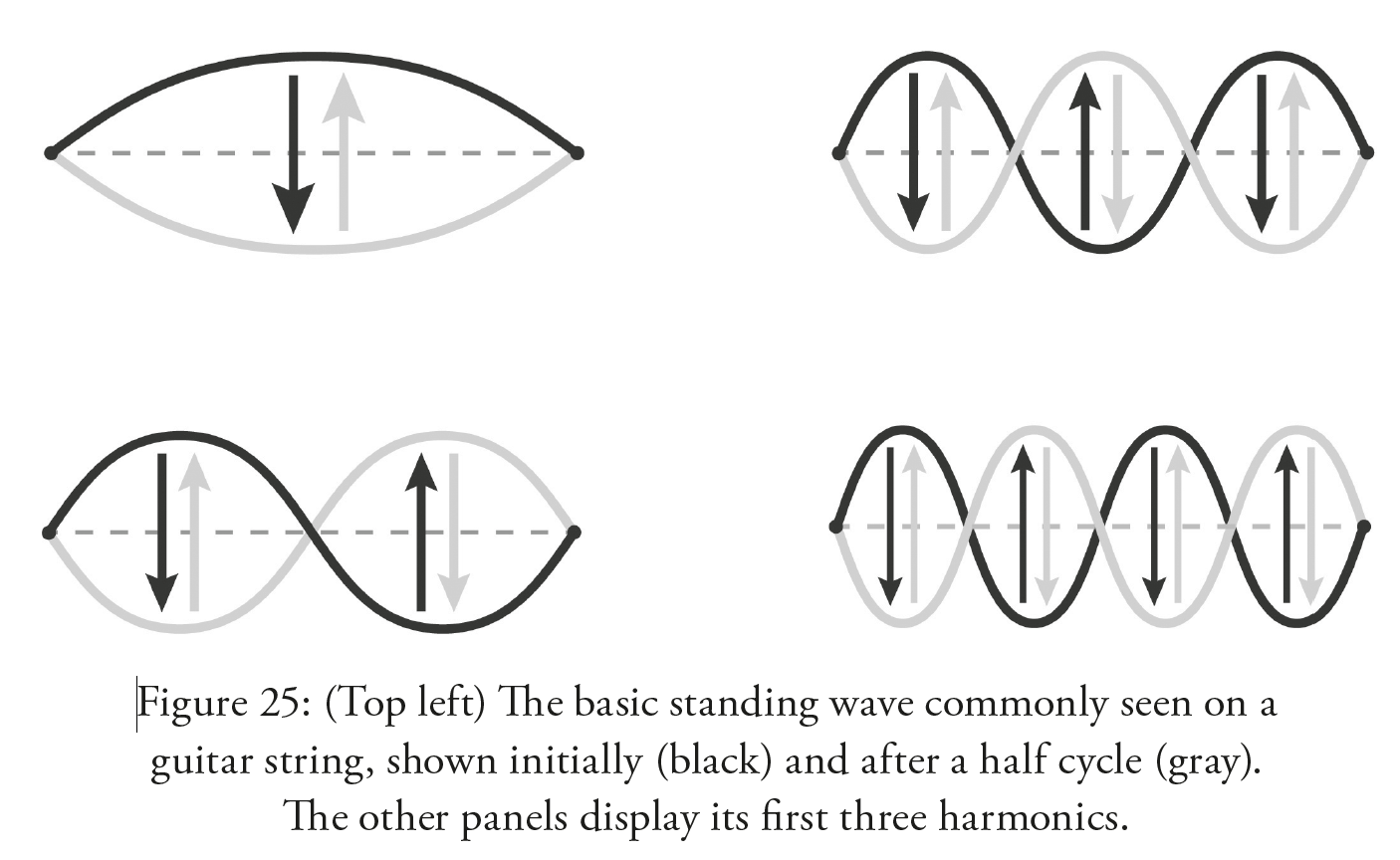
Familiar Standing Waves

A string or other extended vibrating object may have many types of standing waves. For a string, the four simplest standing waves are shown below (Figure 25 from the book chapter 11; illustration by C. Cesarotti).

But we can just focus our attention on the simplest of all such waves, the one at upper left, which has a single crest that over time becomes a single trough and back again, over and over.

The simplest standing wave on a string (in green) of finite length; the dashed line shows where the string would be located in the absence of a wave.

Classic examples of these simplest standing waves are found on the strings of guitars and pianos; somewhat similar waves are found in organ pipes and flutes. As budding musicians quickly learn, it’s generally the case that the longer the string or pipe or bell, the lower the frequency of the wave and the lower the musical note. An organ’s lowest notes come from its longest pipes, and shortening a guitar string with your finger causes the instrument to create a higher note.

[It’s not quite as simple as that because, as covered in chapter 10, there are other ways to change frequency; tightening a string raises it, while replacing air with another gas can raise or lower it. But for a fixed material with fixed properties, what I’ve said is true.]

A simple version of this basic idea is illustrated by taking a box whose sides are of length , filling it with some sort of material, and considering that material’s simplest standing wave. For most familiar materials, the frequency of the standing wave decreases as the length of the box increases; specifically, if you double the length of the box, the frequency drops in half. Thus frequency is inversely proportional to length, as it is on many musical instruments, and as the box’s size becomes infinite, no standing wave remains — its frequency becomes zero, meaning that it no longer vibrates at all.

[In math, we would write

• ,

where is the speed with which traveling waves can move across the substance.]

Unfamiliar Standing Waves

However, there are other standing waves whose frequency of vibration does not decrease in this way. For standing waves of this unfamiliar sort, doubling the length of the box does not cause the frequency to drop in half. In fact, if the box is big enough, doubling its size barely has any effect on the frequency at all! (This can happen in unfamiliar materials, or in familiar materials treated in unusual ways; see chapter 20.2 for a couple of examples.)

If you put one of these unfamiliar standing waves in a box and make the box larger and larger, its frequency won’t drop all the way to zero. Instead it will settle down to a steady frequency, which I’ll label and refer to as the “resonance frequency”. No matter how big the box, the smallest the wave’s frequency can possibly be is the resonance frequency . Said another way, if is sufficiently large, the difference between and will be too small to notice, or even to measure.

[In math, the wave’s frequency is related to the resonance frequency and to the length of the box by an equation similar to

The precise form of the expression depends on details of the box and the vibrating material; but the details are not important here.]

Summarizing the Two Waves

The size and shape of a large box thus affects these two types of standing waves differently,

• impacting the shape and the frequency of familiar standing waves, while
  
  
• impacting the shape of unfamiliar standing waves, but not their frequency

This difference is illustrated in animations found here, and in the graph below, which shows how the frequencies of familiar and unfamiliar standing waves depend on the length of the box.

The frequencies of familiar standing waves (blue) decrease down to zero as L goes to infinity, but those of unfamiliar standing waves (orange) never go below a non-zero minimum frequency f0. A Wave that Stands Without Support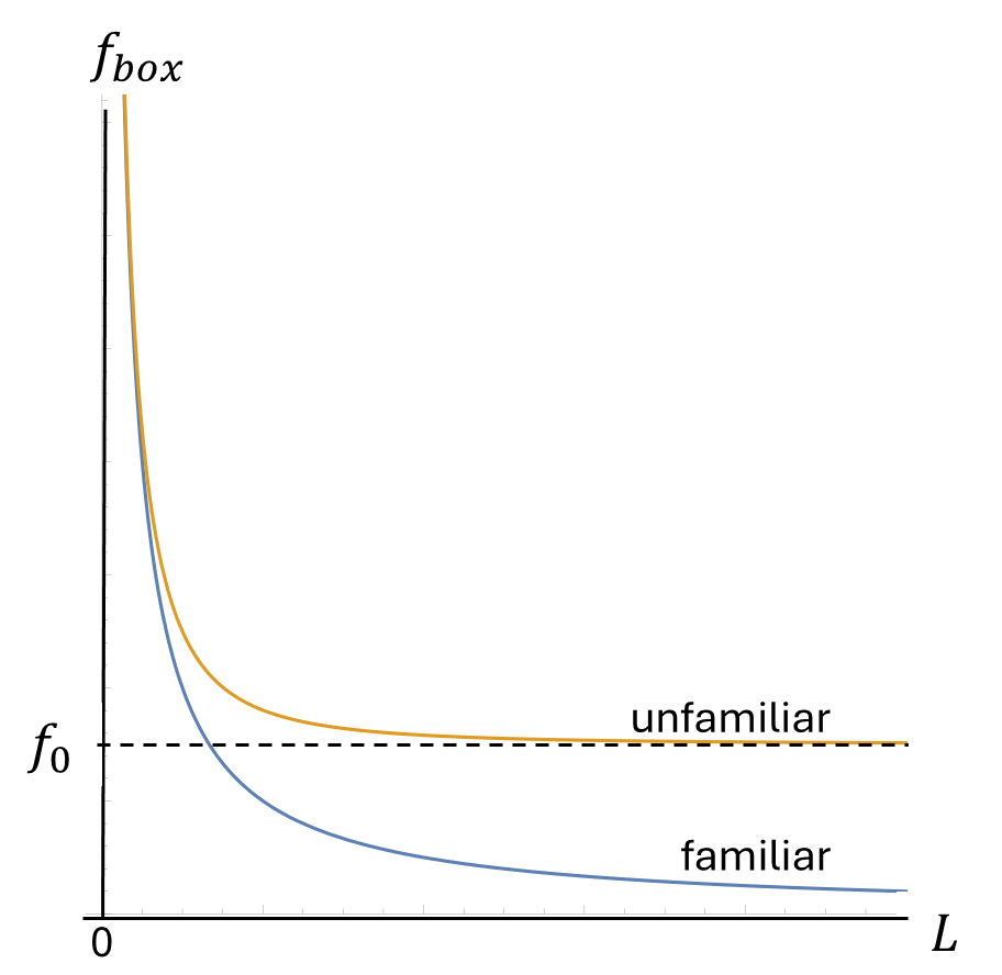

Suppose, then, that we take an unfamiliar standing wave and dismantle its box, or let its box grow to infinite size. Do we then have a standing wave that stretches all across the entire universe?! Well, mathematically speaking, this would indeed be true. But in realistic situations, the standing wave will always run into some obstructions around its edges. Perhaps your hand is close by, as is the ground and a nearby wall; trees and mountains block the wave in other directions, and so forth. Even out in deep space, the space is not completely empty; there are always stray particles moving by.

These objects will affect the shape of the standing wave. But if they are far enough away from the core of the standing wave, they do not affect its frequency — at least, not by an amount that anyone could readily notice or measure.

Thus even a realistic standing wave, with a diameter far smaller than the size of the universe, will vibrate at its resonance frequency if it is sufficiently isolated. That’s more than enough for the purposes of the universe.

The Importance of These Waves

And so an isolated, stationary electron corresponds to an unfamiliar standing wave whose shape is determined by its local environment, but whose frequency is not. It will vibrate at the same rate whether it is in deep space far from any stars, or whether it is in an empty, airless box the size of a sugar cube.

Why should we care? Because there is a direct connection between the frequency of this standing wave and the electron’s rest mass. Explaining that connection is the most important goal of the first two-thirds of the book (through chapter 18). In addition, there’s a link between this issue and the Higgs field — a topic of the book’s remainder (especially chapter 20.)

I hope I’ve managed to write this post in a way which is useful even if you aren’t reading the book. For those reading it, it may well be helpful in clarifying chapters 17-20, where these issues take center stage. If you have found this post confusing, please leave comments, or ask a question on my new Book Questions page. As always, your questions and suggestions will help me improve this website.

About a month ago, there was a lot of noise, discussion and controversy concerning CERN‘s proposal to build a giant new tunnel and put powerful new particle accelerators in it. This proposal is collectively called the Future Circular Collider (“FCC”). (The BBC reported on it here.)

Some scientists made arguments that FCC is a great idea, based on reasoning that I somewhat disagree with. Others said it would be a waste of money, based on reasoning that I again disagree with. But any decision on whether to actually fund the building of the FCC’s tunnel is still some years off, so I was reluctant to get involved in the debate, especially since my nuanced opinion seemed likely to be drowned out amid the polemics.

But I did eventually write something in response to a reporter’s questions, and looking back on it, I think it may be of interest to some readers. So here it is.

My Opinions on the FCC

My starting point is the timeline for the machine.  Quoting from the FCC website, we are looking at “start of construction after the middle 2030s, with the first step of an electron-positron collider (FCC-ee) beginning operations around 2045. A second machine, colliding protons (FCC-hh) in the same tunnel, would extend the research programme from the 2070s to the end of the century.”

Now, although they use the same tunnel, these are two utterly different colliders, with complementary goals.  It’s extremely useful to compare these plans with the journey of CERN from 1985 to 2035, which the FCC is designed to repeat.

The Previous Five Decades: One Tunnel, Two Machines

In the latter 1980s, a 27 km (17 mile) near-circular tunnel was built under the French and Swiss countryside around CERN. Over the decades, two entirely different machines were built in that tunnel:

1.  LEP, an electron-positron collider, which itself had two stages:
   • LEP-1, which created electron-positron collisions with energy-per-collision just below 100 GeV. A high-precision, targeted machine, it was intended to study the Z boson in great detail, and allow searches for possible rare phenomena involving particles of lower mass.
   • LEP-2, an upgrade to LEP-1, gradually pushed the collision energy up to 209 GeV. Somewhere between targeted and exploratory, it was used to study the W boson in detail, and to search for the particle known as the “Higgs boson” to the extent that it could. 
     
2. LHC, a proton-proton machine with a collision energy of 7000 – 14000 GeV, had a largely different goal. A fully exploratory machine, it was aimed mainly at unknown particles. In particular, it was intended to search for the Higgs boson (or whatever might have taken its place in nature), as well as for other particles that might be loosely associated with the Higgs boson. And it could search for many other types of particles too; hence the long lists of published experimental searches (such as this one).

Again, although LEP and LHC occupied the same tunnel and were operated by many of the same people, they were completely different machines that shared little else. 

The Next Five Decades: One Tunnel, Two Machines

In largely the same way, the proposal is for the FCC tunnel to be used for two completely different machines analogous to LEP and LHC. 

• Phase 1) FCC-ee, a more powerful version of LEP, comes first and is a targeted machine at relatively low energy (electron-positron collisions at 100-365 GeV, depending on the target, but with a very high collision rate — up to a hundred thousand times more than LEP-1.)  Its most important target is the Higgs boson, but it also would carry out detailed studies of the Z boson, W boson, and the top quark.
  
  
• Phase 2) After FCC-ee has operated for a long time and collected lots of data, the current plan is that it would be dismantled, and the FCC-hh would be built inside the same tunnel. This machine would be a proton-proton collider like the LHC, only much more powerful, with up to 7 times the energy-per-collision. Like the LHC, it would be an exploratory machine: a general-purpose device that can search for a great variety of unknown particles and phenomena. 

To Focus on Phase 2 is Premature

Let’s work backwards from Phase 2. What are the goals for the FCC-hh?

Asking physicists of today to state a precise goal for such a distant future is somewhat like asking Oppenheimer, all the way back in the 1950s, to predict the main aims of the LHC!  It’s too early to expect a reliable answer. I suspect that current speculation about what the main motivation for FCC-hh will actually be, four or five decades from now, is likely to be wrong.  (That said, there are some specific questions about the Higgs boson and Higgs field that only FCC-hh can address — most notably, how the Higgs field interacts with itself.)

Of course, I do understand why people are talking about FCC-hh right now. If CERN is going to build such a large tunnel, they ought to have some sensible ideas as to how it could be used not only soon but well into the distant future.

But nevertheless, a final decision on FCC-hh — whether and when to build it, and what its goals should be — lies decades away.  It’s Phase 1 that really matters now.  And Phase 1 has a clear purpose and a clear motivation.

Only Phase 1 (FCC-ee) Matters Right Now

What good is FCC-ee? You might well wonder! Since LHC has already run proton-proton collisions at 14000 GeV, making it capable of creating certain types of particles whose masses are several times larger than the Higgs boson or top quark, what hope do we have that FCC-ee, at a much, much lower collision energy, could make any new discoveries? 

The answers are analogous to the ones that were appropriate for LEP-1, whose collision energies were already below those of the Tevatron, a predecessor to the LHC.

• First, FCC-ee can make precision studies of large numbers of Higgs bosons (and enormous numbers of Z bosons). These studies might uncover small cracks in the Standard Model — small deviations from its predictions — giving a first clue that new phenomena are present that are either (a) at higher energy than LHC can reach or (b) too rare and/or obscure for LHC to discover.  FCC-ee might not reveal any details of these novel phenomena, but it would teach us that something new was within reach.  In this case, the FCC-hh would be the ideal exploratory machine to follow FCC-ee. That’s because, compared to LHC, it can both reach higher in energy and produce lower-energy processes at a higher rate, giving it many avenues in which to search for the causes of the above-mentioned cracks.
  
  
• Second, FCC-ee can search for new particles of lower mass than the Higgs boson. Such particles could have been missed by LEP and the LHC if they are produced too rarely, or if they are somehow obscured in the busy environment of the LHC’s proton-proton collisions.  Collisions in an electron-positron machine are much more pristine, and more easily reveal odd or rare phenomena. For instance, both the Z boson and Higgs boson might potentially decay to what are known as “dark” or “hidden” particles, which can be very difficult for the LHC experiments to observe.  If such particles were discovered in Phase 1, then, depending on those particles’ details, one might well modify the plans for Phase 2. (For instance, certain types of dark/hidden particles would be difficult for FCC-hh to study, and might motivate a different Phase 2.)

The rationale for building FCC-ee is very clear: to take full advantage of what the Higgs boson and its field can teach us. Only recently discovered, the Higgs boson is unique among the known elementary particles as the only particle that has no “spin” — no intrinsic angular momentum — and as the particle whose interactions with other particles are most diverse in strength. The corresponding Higgs field, which gives electrons their mass and makes atoms possible, is even more important: it’s crucial for planets and for life. 

Our knowledge of this field and its particle will still be very limited even when the LHC shuts down for good around 2035. Few of the LHC’s measurements of the Higgs boson’s properties will be precise, and some properties simply will not be measurable.  For all we will know in 2035, it could still be the case that one in every twenty Higgs bosons decays to particles that are currently unknown; the LHC experiments will be unable to rule out this possibility.  The FCC-ee will change this, making far more measurements, bringing much higher precision to many of them, and allowing searches for decays to particles that LHC has no hope of observing.

Thus FCC-ee will give us a better handle on the properties of the Higgs boson and Higgs field than the LHC can achieve, and allow us access to rare and/or obscure phenomena that LHC experiments cannot discover.  The potential significance of these scientific advances should not be underestimated.

The FCC-hh of Phase 2 is for the distant future. It will depend crucially on whether Phase 1 finds something, and on what it finds.  It also depends on the results of many other smaller-scale experiments which will be running over the next 35 years.  Any particle physics discovery before 2060 will influence the way we think about the goals of FCC-hh, and so I view it as far too early to wax poetic about what Phase 2 could do, or to criticize it as a waste of money.  We can have that debate over the next generation.  

By contrast, the goals of FCC-ee are clear, and the cost and benefits easier to identify.  That’s why, in my opinion, Phase 1 is the only topic worthy of serious discussion and debate right now.

I’m aiming to get the blog back to science as soon as possible, but I need to answer some questions that I’ve been receiving about the book and website.

• Yes, there will be an audiobook. It’s coming. A few weeks. I’ll let you know.
• Yes, there will be a page on this website where book-readers can ask questions about the subjects covered in the book. No later than next week. I doubt I’ll be able to answer all questions individually, but I’ll be collecting them and answering the most common… see below.

In fact, there will soon be a whole wing of this website devoted to the book, which will have

• Growing lists of Frequently Asked Questions [FAQs], based on readers’ comments and queries
• Expanded discussion of a number of subjects that didn’t fit into the book
• For those who like math (which the book avoids), some of the technical details behind key topics
• A list of figures to refer to when listening to the book (in fact you can already check out that page)
• Animations of some of the figures, aiming to make them clearer than a still image
• A newsletter for those who want to stay up to date on upcoming events

And more! [Some parts of this are almost ready, but we’re delayed by an array of minor technical issues with the newly upgraded website. Hopefully in a week or two.]

Speaking more broadly, the new book is just a part of a much larger project: to convey the worldview of contemporary physics to as many people as possible, making it accessible without watering it down. I hope to make it as clear as it can be made, and as meaningful. But the book, no matter how hard I have worked at it or how successful I may or may not have been at writing it, cannot possibly do that alone. Hence the commitment to expand the website, answer your questions, give public talks and courses, and much more to come.

By the way, the second half of the conversation with Daniel Whiteson on his podcast is posted. (Here’s the first half; and here’s the conversation on Sean Carroll’s podcast.)

Recently, a reader raised a couple of central questions about speed and relativity. Since the answers are crucial to an understanding of Einstein’s relativity in particular and of the cosmos in general, I thought I’d bring them to your attention, in case you’ve had similar questions.

The Questions

I understand that the vacuum speed of light [“c“] is constant throughout the Universe, and I’m familiar with the math that shows that the energy required to accelerate a particle becomes infinite as the speed approaches c. But what physical effect enforces this behavior? If a proton, for example, gets ejected in a supernova explosion, how does it “know” that it’s getting close to c and can’t go any faster?

And as a corollary to this question, what is the reference frame for measuring these relativistic velocities? For example, when a particle beam at CERN is said to be moving at 99.99% the speed of light, is that speed relative to the infrastructure at CERN? Or does it somehow account for the velocity components that arise from the rotation of the Earth, the orbital motion of the Earth around the Sun, the galactic motion of the Sun in the Milky Way, and so on?…

The Answers The Oblivious Proton

How does a proton know that it is getting close to c and can’t go any faster? It doesn’t.

For the same reason, you, too, right here and now, have no sense of how fast you are moving.

• If a proton is moving at a constant speed, and not accelerating, then as far as it can tell, it is stationary. It “feels” just as stationary, flying across our galaxy at nearly c, as you and I do, carried around the spinning galaxy at about 0.1% of c (150 miles per second).
  
• If the proton is accelerating, it will indeed “feel” the acceleration, in that its internal structure will potentially respond to its changing speed. But even so, it has no idea how fast it is going, so it can’t possibly worry its little head about exceeding c. . .any more than you and I do.

Absolute Speed

Implicitly, in asking these questions, you are holding in your mind a notion of “absolute speed.” You are imagining that the proton has a real, honest, unambiguous true speed, and it is this absolute speed that can’t exceed c.

But even Galileo, nearly 400 years ago, would have suggested to you that your notion of “absolute speed” is suspect. After all, we are in extremely rapid motion relative to the Earth’s center, the Sun, the galaxy, and yet we feel nothing… and indeed, we only know about our various motions by a series of complex arguments and measurements in astronomy. There’s no way to go into a closed room and measure that we are moving around the galaxy at 150 miles per second. Absolute speed cannot be measured by any experiment. This is for a simple reason: absolute speed does not exist in our universe. The notion is meaningless.

The meaninglessness of absolute speed is nothing less than the principle of relativity, as stated by Galileo in 1632, and as preserved by Einstein in his work of the early 1900s.

The problem with the question, “what is the reference frame for measuring these relativistic velocities”, is that it presumes that there is a preferred reference frame relative to which absolute velocities have meaning. But both Galileo and Einstein tell you to banish the thought.

Relative speed

ALL velocities in our universe are relative. There are no absolute velocities. Einstein’s statement about “objects moving at speeds slower than or equal to c” is not about absolute velocities at all — because there are no such things. So what, in fact, does he mean?

Einstein’s statement is the following: when two objects pass one another, then the speed of the first object as measured by an experiment moving along with the second object — a relative speed!!! — must be less than c. There’s one sole exception: if the first object has zero rest mass and is moving through empty space, then the relative speed (of the first object as measured by the experiment moving with the second object) is exactly c.

An aside: as discussed in this post, if one object passes me to the left at 0.99 c, and a second passes me to the right at 0.99c, their relative speed, as I measure it, is greater than c — it is indeed 1.98 c. But Einstein makes no statement about how an observer views the motion of two objects relative to each other. His statement is about an observer views the motion of one object relative to the observer; only that relative speed must be less than or equal to c.

You see how crucial it is to get the details exactly right. Otherwise paradoxes, such as those implicit in the reader’s original questions, loom everywhere. Indeed, if we try to make sense of Einstein’s statements using our familiar notions of space and time, we will immediately find contradictions that we cannot resolve. Einstein’s great leap of genius was to realize that once we understand that space and time can vary, in precisely the way that they do in his updated notion of Galileo’s relativity, all the apparent paradoxes are eliminated.

The Particle Beams at CERN

when a particle beam at CERN is said to be moving at 99.99% the speed of light, is that speed relative to the infrastructure at CERN?

Yes, typically that’s what a person making that statement implicitly means; the speed of the beam is typically measured relative to the CERN laboratory. But that’s a choice, made out of convenience. By contrast,

• A person flying by CERN at a relative speed of 99.99% of c, moving in the same direction as the particle beam, would see the particles as stationary.
• Meanwhile a person moving in the opposite direction of the beam at 99.99% of c relative to CERN would see the particles moving at 99.9999995% of c.

Who is right? Everyone. Speed is relative; and when something is relative, everyone disagrees, yet no one is wrong.

In summary, a proton does not need to know, and cannot know, its absolute speed. Instead, what Einstein’s view of relativity says is this: no matter how observers are moving around, they will always find that a passing proton’s speed, as measured relative to themselves, is less than c.

[Comments may not yet be working for all readers for this post; sorry for the technical issue! We hope to have the system working a bit later today, so if your attempt to comment fails, please save your questions and thoughts until we’re back on track.]

You're currently a free subscriber. Upgrade your subscription to get access to the rest of this post and other paid-subscriber only content.

Upgrade subscription

How confident can we be that light’s speed across the universe is really constant, as I assumed in a recent post? Well, aspects of that idea can be verified experimentally. For instance, the hypothesis that light at all frequencies travels at the same speed can be checked. Today I’ll show you one way that it’s done; it’s particularly straightforward and easy to interpret.

LHAASO and Photons

Light’s speed in empty space is widely thought to be set by a universal cosmic speed limit, c, which is roughly 300,000 km [186,000 miles] per second. Over time, experiments have tested this hypothesis with ever better precision.

A recent check comes from the LHAASO experiment in Tibet — LHAASO stands for “Large High Altitude Air Shower Observatory” — which is designed to measure “cosmic rays.” A cosmic ray is a general term, meaning “any high-energy particle from outer space.” It’s common for a cosmic ray, when reaching the Earth’s atmosphere, to hit an atom and create a shower of lower-energy particles. LHAASO can observe and measure the particles in that shower, and work backwards to infer the original cosmic ray’s energy. Among the most common cosmic rays seen at LHAASO are “gamma-ray photons.”

Light waves vibrating with slightly higher frequency than our eyes can detect are called “ultra-violet”; at even higher frequencies are found “X-rays” and then “gamma-rays.” Despite the various names, all of these waves are really of exactly the same type, just vibrating at different rates. Moreover, all such waves are made from photons — the particles of light, whose energy is always proportional to their frequency. That means that ultra-high-frequency light is made from ultra-high-energy photons, and it is these “gamma-ray photons” from outer space that LHAASO detects and measures.

A Bright, Long-Duration Gamma-Ray Burst

In late 2022, there was a brilliant, energetic flare-up — a “gamma-ray burst”, or GRB — from an object roughly 2 billion light-years away (i.e., it took light from that burst about 2 billion years to reach Earth.) We don’t know exactly how far away the object is, and so we don’t know exactly when this event took place or exactly how long the light traveled for. But we do know that

• if the speed of light is always equal to the cosmic speed limit, and
• if the cosmic speed limit is indeed a constant that is independent of an object’s energy, frequency, or anything else,

then all of the light from that GRB — all of the gamma-ray photons that were emitted by it — should have taken the same amount of time to reach Earth.

This GRB event was not a sudden flash, though. Instead, it was a long process, with a run-up, a peak, and then a gradual dimming. In fact, LHAASO observed showers from the GRB’s photons for more than an hour, which is very unusual!

As discussed in their recent paper, when the LHAASO experimenters take the thousands of photons that they detected during the GRB, and they separate them into ten energy ranges (equivalent to ten frequency ranges, since a photon’s energy is proportional to its frequency) and look at the rate at which photons in those energy ranges were observed over time, they find the black curves shown in the figure below. LHAASO’s data is in black; the names “Seg0”, etc, refer to the different ranges; and the vertical dashed line was added by me.

Black curves show the rates at which photons in ten different energy ranges were observed by LHAASO during a 300 second period in which the GRB was at its brightest. I have added a vertical dashed line to show that all ten peaks line up in time. The approximate energies of the ranges, shown at right, are taken from the LHAASO paper, which you should read for further details.

In units of 1 TeV (about 1000 times the energy stored in the E=mc2 energy of a single hydrogen atom, and about 1/14th of the energy of each collision at the Large Hadron Collider), LHAASO was able to observe photons with energy between roughly 0.2 TeV and 1.7 TeV. Looking at the rate at which photons of different energies arrived at LHAASO, one sees that the peak brightness of the GRB occurred at the same time in each energy range. If the photons at different energies had traveled at different speeds, the peaks would have occurred at different times, just as sprinters with different speeds finish a race at different times. Since the peaks are roughly simultaneous, we can draw some conclusions about how similar the speeds of the photons must have been. Let’s do it!

Light’s Speed Does Not Depend on its Frequency

We’ll do a quick estimate; the LHAASO folks, of course, do a much more careful job.

From the vertical dashed line, you can see that all ten peaks in LHAASO’s data occurred at the same time to within, say, 10 seconds or better. That means that at the moment the GRB was brightest, the photons in each of these energy ranges

• left the source of the GRB,
• traveled for about 2 billion years, and
• arrived on Earth within 10 seconds of each other.

Since a year has about 30 million seconds in it, 2 billion years is about 60 million billion seconds (i.e. 6 times 1016 seconds.) And so, to arrive within 10 seconds of one another, these photons, whose energies range over a factor of about 5, must have had the same speed to one part in 6 million billion. Said another way, any variation in light’s speed across these frequencies of light can be no larger than, roughly,

• 10 seconds / 2 billion years = 10 seconds / ([2 x 109 years] x [3×107 seconds/year])
  = 10 seconds /(6 x 1016 seconds) = 2 x 10-16 !

Notice we do not need a precise measurement of the photons’ total travel time to reach this conclusion.

The LHAASO experimenters do a proper statistical analysis of all of their data, including the shapes of the ten curves, and they get significantly more precise results than our little estimate. They then use those results to constrain specific speculative theories that propose that the speed of light might not, in fact, be the same for all frequencies. If you’re interested in those details, you can read about them in their paper (or ask me more about them in the comments).

Bottom Line

LHAASO thus joins a long list of experiments that have addressed the constancy of the speed of light. Specifically, it shows that when light of various high frequencies (made up of photons of various high energies) travels a very long distance, the different photons take exactly the same amount of time to make the trip, as far as our best measurements can tell. That’s strong evidence in favor of our best guess: that there is a cosmic speed limit that holds sway in the universe, and that light traveling across the emptiness of deep space always moves at the limit.

And yet… it’s not final evidence. Grand scientific principles can never be permanently settled, because all experiments have their limitations, and no experiment can ever deliver 100%-airtight proof. Better and more precise measurements are still to come. Maybe one of them, someday, will surprise us…?

Quick note today: I’m pleased and honored to share with you that the world-renowned journal Science has published a review of my upcoming book!

The book, Waves in an Impossible Sea, appears in stores in just 10 days (and can be pre-ordered now.) It’s a non-technical account of how Einstein’s relativity and quantum physics come together to make the world of daily experience — and how the Higgs field makes it all possible.

Nothing goes faster than the speed of light in empty space, also known as the cosmic speed limit c. Right? Well, umm… the devil is in the details.

Here are some of those details:

1. If you hold two flashlights and point them in opposite directions, the speed at which the two beams rush apart, from your perspective, is indeed twice the cosmic speed limit.
2. In an expanding universe, the distance between you and a retreating flash of light can increase faster than the cosmic speed limit.
3. The location where two measuring sticks cross one another can potentially move faster than the cosmic speed limit.

I addressed issue #1 in a blog post last year.

Today I’ve just put up an article on issue #2. (This is a part of my effort to expand on loose ends raised in the footnotes from my upcoming book).

As for issue #3, can you see why it might be true?

If you aren’t sure and want the answer, click here:

The “location where two measuring sticks meet” is not itself an object. Only objects — localized material things with energy and momentum — are constrained to have relative speeds below the cosmic speed limit — and even that statement needs to be made more precisely (see detail #1 above!) A meeting point between objects is not itself an object, and may move faster than c even if the objects move slower than c. The figure below illustrates this.

One stick is shown in black, the other in red. The red one then moves downward; the dotted line shows where it was initially. Although the red stick moves only a short distance during the animation, the meeting point of the two sticks crosses the entire animation from left to right. If the red stick is moving at half the cosmic speed limit, which is perfectly consistent with Einstein’s relativity, the meeting point, which covers much more ground in the same amount of time, is clearly moving faster than the cosmic speed limit. No problem: no thing moved faster than the speed of light.

One stick (black) moves downward, starting from the dotted line, and passing another stick(red). The speed at which their crossing point moves is much faster than the speed of the moving stick itself. While the black stick cannot move faster than the cosmic speed limit relative to the red stick, their crossing point can do so.

Note added: in materials, the speed of light is generally slower than the cosmic speed limit. For this reason, objects inside materials can move faster than the speed of light but slower than the cosmic speed limit. The result is a very interesting and useful effect: Cerenkov radiation, widely used in particle physics experiments such as Ice Cube!

I have posted my fourth article discussing zero-point energy. (Here are the first, the second, and the third, which covered respectively the zero-point energy of a ball on a spring, a guitar string, and a bosonic field whose particles have zero mass, such as the electromagnetic field.) Today’s article looks at fields whose particles have non-zero mass, such as the Higgs field, and fermionic fields, such as the electron field and quark fields. It presents some simple formulas, and in its final section, shows how one can obtain them using math.

Along the way we’ll encounter the idea of “supersymmetry” and its failed role in the cosmological constant problem. This is a word which (for some good historical reasons) generates a lot of heat. But stay calm; I’m neither promoting it nor bashing it. Supersymmetry is an idea which proves useful as a conceptual tool, whether it is true in nature or not.

So that you know where I’m headed: after this article, we’ll now be in a position to understand (using only simple formulas) where the hierarchy puzzle comes from and why it is tied up with the concept of zero-point energy. Then, finally, we can grasp what’s puzzling about the hierarchy, and look at various proposed solutions to it, ranging from fancy math to historical drama, or even denying that it’s puzzling at all.

My two new webpages from earlier this week addressed the zero-point energy for the simple case of a ball on a spring and for the much richer case of a guitar string; the latter served as a warmup to today’s webpage, the third in this series, which explains the zero-point energy of a field of the universe. This subject will lead us head-first into the cosmological constant problem. As before, the article starts with a non-mathematical overview, and then obtains the results stated in the overview using pre-university math (except for one aside.) [As always, please comment if you spot typos or find some of the presentation especially confusing!]

(See the first post announcing this series for a brief summary of the hierarchy puzzle, which motivates this whole series, and for links to longer related discussions of it.)

The next webpage after this one will be an extension to today’s, covering other types of fields. That will lead us deeper into the cosmological constant problem, and begin to touch on the hierarchy puzzle.

In my last post, I introduced a new webpage concerning “zero-point energy”, the core concept that lies at the heart of the hierarchy puzzle. I have now posted the next webpage in the series, which extends the notion of zero-point energy to a slightly more complex system, an ordinary metal string of finite length. It’s a bit schematic, but it serves to teach us some crucial and surprising lessons about the zero-point energy associated with the internal vibrations of physical objects. [Please let me know in the comments if you spot any typos or if you find some of the presentation especially confusing!]

(See the previous post for a brief summary of the hierarchy puzzle, and for links to longer discussions of it.)

The next webpage to come will apply these lessons to quantum fields themselves. Then things will really become interesting — directly and profoundly relevant to the universe as a whole.

A central issue in discussions of particle physics’ present and future is known as the hierarchy puzzle. Although I discuss the hierarchy — its confusing nature and the debates that it generates — in my upcoming book, I do so rather briefly, and so, I’ll be putting up some new pages on this website with supplemental information. The same information is relevant for the cosmological constant problem. (Older pages already giving various perspectives on these issues can be found here, here and here.)

I have just posted the first new page, on “zero-point motion” and “zero-point energy.” It begins with a verbal, non-technical description of zero-point motion and zero-point energy. There follows a sketch of the details using pre-university math. Future pages will apply these ideas to quantum fields, addressing notions of “vacuum energy density” and the “cosmological constant”, and then turning to “Higgs feedback” and the core of the hierarchy puzzle.

A quick description of the hierarchy in question: it is a hierarchy of energy scales, or of mass scales. One way it can be described is in terms of particle masses:

• The masses [meaning “rest masses”] of all elementary particles are absurdly small compared to the Planck mass, the lowest possible mass for a black hole

The masses of the known elementary particles lie between 200 times larger or 2000 smaller than a proton’s mass, excepting neutrinos’ masses, which are even smaller, and the zero rest mass of photons, gluons, and (presumed) gravitons. But if our understanding of gravity is taken at face value (and maybe it should not be), the smallest possible black hole would have a mass of at least a billion billion protons.

Alternatively, we may rephrase the hierarchy in terms of forces:

• For all known elementary particles, gravity is astonishingly weak compared to the other elementary forces.

The strong nuclear force, acting on the quarks inside of protons, is about as strong as a force can possibly be; electromagnetism’s strength is about 1% of that; but gravity’s effects on a proton are a billion billion times smaller than that of the strong nuclear force.

The origin of the hierarchy is unknown. What makes the hierarchy puzzling is that when we look at the particles we know, organized in what is called the Standard Model of Particle Physics, it seems highly non-generic. If we consider the Standard Model not in isolation but as a representative of a large class of similar possible universes, it is unusual, in that almost all universes of similar type would have no such hierarchy. In most such theories, masses would either be zero or huge. To be precise, some particles might have no mass at all, while all others would have masses near the Planck scale — and for the latter, gravity would be as strong as the other forces.

Of course, we only live in one universe, and it doesn’t have to be generic. But in the past, when we’ve found an aspect of the universe that’s highly non-generic, there has usually been a story behind it — and so, on heuristic grounds, one might suspect that this gigantic and non-generic hierarchy might point toward some important facts about the universe that we still don’t know. The questions of how much weight to give that suspicion, and of whether the missing facts might lie within close experimental reach, is one we can return to after I’ve fully laid out the underlying scientific issues.

Last night, using the methods I described as part of my check-it-yourself astronomy series, I estimated the distance to the planet Jupiter using nothing more than my eyes, a protractor, and a simple calculator. It took about 30 seconds of measuring something before and after sunset, and about 15 more seconds using my cell phone’s calculator. You can do it too, if you have clear skies over the weekend.

There are only two parts of the process:

1. know which week to ask the question, and
2. during that week, measure the angle A in the sky between the Sun and Jupiter.

Then the distance from Jupiter to the Sun RJS is the distance from Earth to the Sun RES times the tangent of the angle A

The reason is simple geometry, corresponding (for a general planet P) to the figure below.

Figure 1: When an outer planet is about 1/4 or 3/4 through its cycle between one opposition and the next, the Earth, Sun and the planet form a right triangle, which allows a quick estimate of its distance RPS from the Sun relative to the Earth-Sun distance RES. When to Measure?

The day on which you should make the measurement is the one when Earth, Jupiter and the Sun make a right triangle as in Figure 1. You can estimate this date quite easily. Once every 13 months or so, Jupiter is at “opposition”, meaning that there is a straight line connecting the Sun, Earth and Jupiter, as at the far left of Figure 1. At opposition, Jupiter is directly overhead at midnight. Let’s call the time between oppositions the length of Jupiter’s cycle. Then, about 1/4 or 3/4 of the way through the cycle, the three heavenly bodies form a right-angle triangle, drawn in Figure 1, and the angle between Jupiter and the Sun as seen from Earth is enough to determine the ratios of the triangle’s sides.

Looking at Figure 1, you can see that if RJS were just a little larger than RES, the angle A would be close to 45 degrees. If RJS were enormously larger than RES, then the angle would be very close to 90 degrees. But wandering into your backyard just after sunset, and looking up, reveals the angle to be much larger than 45 degrees, yet clearly less than 90.

Figure 2: Last night, 30 minutes after sunset, Jupiter was close to overhead, about 75 or so degrees from the point where the Sun had set, to the right of the image. How to Measure?

This is a bit harder, but how hard it is depends on how accurate an answer you are seeking.

The first problem is that you can’t see Jupiter at the same time you see the Sun — the former is too dim and the latter too bright — so you can’t measure the angle between them directly. You need to watch where the Sun sets. Call that the “sunset point”. Then you need to measure the angle between Jupiter and that point of sunset, let’s say, 30 minutes after sunset. Next, you need on an additional angle that accounts for how far the Sun has moved below the horizon during that 30 minutes. (Perhaps the best way to do this is to look at the Sun 30 minutes before sunset, estimate its angle away from the sunset point, and then, assuming the Sun moves by that same angle in the next 30 minutes, add that angle on to your 30-minutes-post-sunset measurement of Jupiter.)

You’re not going to get a perfectly precise answer, and that leads to the second problem. RJS is quite sensitive to the angle A — the further out the planet is from the Sun, the worse this problem becomes. So if you don’t measure the angle accurately, your estimate of RJS may be rather far off. (Note: Even if you do measure the angle accurately, this method cannot get you a precise answer, because the whole method is based on idealizing Earth and Jupiter as traveling at constant speeds on circular orbits, which is it an approximation of the truth.) This can be seen in the graph below, which shows that as A approaches 90 degrees, the inferred planetary-sun distance grows very rapidly.

Figure 3: The relation between a planet’s distance from the Sun, relative to Earth’s, and the angle that it forms relative to the Sun at the 1/4 or 3/4 stage of its cycle between oppositions. The further is the planet from the Sun, the more precisely the angle must be measured to obtain a good estimate of its distance. My Estimates

I started with a rough qualitative estimate, with no intention to be precise. Just a quick glance at the sky revealed that the angle between Jupiter and the point of sunset was less than 80 degrees and more than 60. Accounting for the Sun’s motion after sunset, that put the angle A between 85 and 65 degrees. That only tells us, as shown in the dashed lines of Figure 4, that the Jupiter-Sun distance lies between 2.2 and 11.6 times the Earth-Sun distance. Still, it already reveals that the ratio of the distances is neither 1.1 nor 100; Jupiter orbit is significantly, though not spectacularly, larger than Earth’s.

Then I measured things a bit more carefully, taking about thirty seconds to do it, and found the estimate shown in the solid lines of Figure 4: the angle is somewhere between 77 and 82 degrees. That’s accurate enough to tell us that RJS lies between 4.3 and 7.1 RES . Although that’s still not precise, it is much better than my first estimate.

Figure 4: My first estimate, given by glancing at the sky, lies between the dashed lines, and determines Jupiter’s position only roughly. My more careful estimate of the angle A lies between the solid lines. The true Jupiter-Sun distance (which varies as Jupiter orbits) is given by the red bar.

In fact Jupiter’s orbit isn’t circular, nor is Earth’s — RJS moves between 4.95 and 5.46 times the average of RES , as shown by the red bar in Figure 4 — so it’s not possible to achieve better than 10%-20% precision using this method. But it’s pretty good for something that requires nothing more than pre-college math and the naked eye! This approach works that much better for Mars (because the angle for Mars is smaller, and the result less sensitive to how well you measure the angle). Conversely, it works less well for Saturn, Uranus or Neptune.

If you like this kind of challenge, try it, and let me know if you succeeded in getting a more precise measurement of the angle and what you found for RJS. Or if you’re a science teacher, give it as a challenge to your students.

A shortcut — less fun, but much more precise — is to look up the positions of Jupiter and the Sun in the sky, using the coordinates on the sky known as “right ascension” and “declination”. This information is easily found on many websites, such as this one and this one. I won’t go into the details here, but it isn’t hard then to extract the angle between Jupiter and the Sun from this information, and obtain a more precise estimate of RJS.

Of course, so far we’ve only found the ratio of two distances, RJS /RES. If we want to know RJS in miles or kilometers, then we need first to measure RES in miles or kilometers. Fortunately, this isn’t that hard to do… using meteor showers. But that’s another story.

Final Thoughts

The distance REJ from Earth to Jupiter changes dramatically as the two planets orbit the Sun, from a maximum of RJS +RES when the planets are on opposite sides of the Sun to RJS –RES when Jupiter is at opposition. But last night, using the right-angle triangle of Figure 1, we know that the distance was given by the secant (=1/cosine) of the angle A:

For angles close to 90 degrees, secant and tangent are almost equal, and so it turns out that my estimate reveals that Jupiter is currently between 4.4 and 7.2 times further away than is the Sun.

With a telescope, there are other methods for obtaining RJS, which you can infer from Figure 1. Jupiter appears larger near opposition, when it is as close as it gets to Earth, and smaller when it lies almost at the other side of the Sun; comparing its angular size at these times would tell you RJS relative to RES . The fraction of the planet which is sunlit from our perspective at various times in the orbit also reveals RJS .

I hope that some of you go out over the weekend and give this a try! It just takes a few minutes. The same approach works for Mars and Saturn, the other naked-eye outer planets, and a similar approach works for Mercury and Venus. But in each case, we have to wait for the right week.

A number of people have asked me my opinion concerning CERN‘s proposal for a new, larger and more powerful particle physics collider… or rather, two completely different colliders that would operate in the same tunnel:

• Phase 1 (two to three decades from now): an electron-positron collider targeted at the detailed physics of Higgs bosons, Z bosons, W bosons and top quarks, using them to search for subtle high-energy phenomena and for rare but dramatic low-energy phenomena;
• Phase 2: (five to six decades from now) an exploratory proton-proton collider, like the Large Hadron Collider [LHC] but with a higher collision energy, and therefore capable of making discoveries of particles that either have higher mass or a lower production rate than what LHC can handle.

Importantly, any decision to fund this machine lies several years away, and in the meantime, a discovery at the LHC or elsewhere might completely change the conversation. So I don’t see the point in writing about this right now.

Instead, I refer you back to my two posts from 2014.

• Why a future 100 TeV collider may make sense
• Why a future 100 TeV collider might not be the best idea

Some details are out of date — time scales are longer, and China is not what it was back then — but much of what I wrote is the same as what I would say today.

My opinion in a nutshell: Phase 1 makes perfect sense to me. Phase 2 seems far less obvious, but it’s decades away, and no final decision has to be made soon.

A couple of years ago I wrote a series of posts (see below) showing how anyone, with a little work, can verify the main facts about the Earth, Moon, Sun and planets. This kind of “Check-It-Yourself” astronomy isn’t necessary, of course, if you trust the scientists who write science textbooks. But it’s good to know you don’t have to trust them, because you can check it on your own, without special equipment.

The ability to “do it yourself” is what makes science, as a belief system, most robust than most other belief systems, past and present. It also explains why there aren’t widely used but competing scientific doctrines that fundamentally disagree about the basics of, say, the Sun and its planets. Although science, like religion, is captured in texts and teachings that have been around for generations, one doesn’t need to have faith in those books, at least when it comes to facts about how the world works nowadays. The books may be from the past, but most of what they describe can be independently verified now. In many cases, this can be done by ordinary people without special training, as long as they have some guidance as to how to do it. The purpose of the “Check-It-Yourself-Astronomy” series is to provide that guidance.

As I showed, nothing more than pre-university geometry, trigonometry, and algebra, along with some star-gazing and a distant friend or two, is required to

• confirm that the Earth’s a spinning (almost-)sphere,
• estimate the size of the Earth and Moon and the distance between them,
• show the Sun’s larger than the Earth and much further than the Moon, and that the stars are further still,
• verify the other planets orbit the Sun and estimate their relative distances from the Sun and their orbital times,
• infer a relation between these distances and times known as Kepler’s law, and show that a similar Kepler-type law works for objects orbiting the Earth,
• infer from these laws that the same gravity that makes ordinary objects fall does so by creating an inward acceleration, one that follows Newton’s inverse square law, holding certain objects in orbit around the Earth and others in orbit around the Sun
• confirm that the Earth orbits the Sun, by invoking Kepler’s law.
  • (Incidentally, this last statement is unambiguous, despite some claims to the contrary, even in Einstein’s theory of gravity.)

However this list is missing something important. From these methods, one can only obtain the ratios of planetary sizes to each other and to the Sun’s size, and the ratios of distances between planets and the Sun. Yet I did not explain how to measure the distance from the Earth to the Sun, or the distance from the Sun to any of the other planets, or the sizes of the other planets. It’s difficult to learn these things without sophisticated equipment and extremely precise measurements; the easiest things to measure about the planets and the Sun — their locations, motions and sizes — aren’t sufficient. (I’ll explain why they’re not sufficient in my next post.)

But shouldn’t there be a way around this problem?

Just One Good Measurement

It shouldn’t be that hard, should it? If we knew any one of these distances or sizes, we could figure out all the others.

For example, in earlier posts we saw how easily one can determine that the ratio of Jupiter’s distance from the Sun to Earth’s distance from the Sun is about 5. [In this paragraph, to keep the argument simple, I use very rough numbers.] Once we learn Earth is about 100 million miles [about 150 million km] from the Sun (which also allows us to compute the Sun’s size), we just multiply this number by 5 to get Jupiter’s distance, about 500 million miles [750 million km] from Earth. That means that Jupiter is about 400 million miles [600 million km] from Earth when the two planets are closest. Then, knowing from a simple backyard telescope that when Jupiter is closest to Earth, and thus 4 times the distance to the Sun, its apparent diameter on the sky is about 1/40 of the Sun’s diameter, we learn that Jupiter’s true diameter is about 4*(1/40) = 1/10 that of the Sun. The same methods can be applied to all the other planets as well as their moons.

The distance between Jupiter and the Sun is about 5 times that of the Earth and Sun, and so, when Jupiter, Earth and the Sun lie in a line, the Jupiter-Earth distance is about 4 times the Earth-Sun distance. This knowledge, combined with the apparent sizes of Jupiter and the Sun, can be used to infer the ratio of Jupiter’s size to that of the Sun. But not one of these sizes or distances is easy to measure. (Not to scale.)

However, finding any one of these distances or sizes is challenging for you and me. A simple geometric method used by Aristarchus in classical Greek times can be used by anyone to prove that that the Sun is at least a few million miles away and thus larger than the Earth. (This in turn tells us that Jupiter is far away and that its size is comparable to or larger than Earth.) But this method does not provide a crisp measurement. It can’t distinguish between the true answer of 100 million miles and a distance of several billion or even several trillion miles.

(Note: Later pre-telescope astronomers claimed a measurement that is only a factor of 2 below the true answer. However, it is not clear to me, from what I’ve read of the historical record, if they truly measured the distance or simply bounded it from below using Artistarchus’ approach, and got lucky that their bound is not far from the real answer. Part of the problem is that estimates of uncertainties are a modern invention; the Greek authors just state a value without any recognition that this value might be wildly off [especially on the high end] simply because of the method used. If any readers have additional insight into this, please let me know. In any case, I am currently unaware of any easy and accurate check-it-yourself method that ancient astronomers could have employed.)

In the 1600s and 1700s, the distances to other nearby planets were determined using difficult parallax measurements, in which a planet was observed carefully at two distant locations (or two different times) on Earth. Modern methods often involve firing a strong radar pulse at another planet, Mars or Venus typically; the pulse reflects off that distant planet, and the arrival time of the faint echo, times the known speed of light (also known as the cosmic speed limit, 186000 miles [300000 km] per second), equals twice Earth’s distance to the planet. As I emphasized above, it only takes one such measurement to fix the distances and sizes of all the distant, large objects in the solar system. Unfortunately, none of these techniques is easily reproduced without highly precise measurements and/or fancy equipment.

Nevertheless, it turns out that there are less well-known methods that, via an indirect route, can get us a good estimate of the distance to the Sun, in ways that don’t suffer from the problems of Artistarchus’ approach. This is what I will explain over the next few posts…