Science blog of a physics theorist Feed

Before we knew about quantum physics, humans thought that if we had a system of two small objects, we could always know where they were located — the first at some position x1, the second at some position x2. And after Isaac Newton’s breakthroughs in the late 17th century, we believed that by combining this information with knowledge of the objects’ motions and the forces acting upon them, we could calculate where they would be in the future.

But in our quantum world, this turns out not to be the case. Instead, in Erwin Schrödinger’s 1925 view of quantum physics, our system of two objects has a wave function which, for every possible x1 and x2 that the objects could have, gives us a complex number Ψ(x1, x2). The absolute-value-squared of that number, |Ψ(x1, x2)|2, is proportional to the probability for finding the first object at position x1 and the second at position x2 — if we actually choose to measure their positions right away. If instead we wait, the wave function will change over time, following Schrödinger’s wave equation. The updated wave function’s square will again tell us the probabilities, at that later time, for finding the objects at those particular positions.

The set of all possible object locations x1 and x2 is what I am calling the “space of possibilities” (also known as the “configuration space”), and the wave function Ψ(x1, x2) is a function on that space of possibilities. In fact, the wave function for any system is a function on the space of that system’s possibilities: for any possible arrangement X of the system, the wave function will give us a complex number Ψ(X).

Drawing a wave function can be tricky. I’ve done it in different ways in different contexts. Interpreting a drawing of a wave function can also be tricky. But it’s helpful to learn how to do it. So in today’s post, I’ll give you three different approaches to depicting the wave function for one of the simplest physical systems: a single object moving along a line. In coming weeks, I’ll give you more examples that you can try to interpret. Once you can read a wave function correctly, then you know your understanding of quantum physics has a good foundation.

For now, everything I’ll do today is in the language of 1920s quantum physics, Schrödinger style. But soon we’ll put this same strategy to work on quantum field theory, the modern language of particle physics — and then many things will change. Familiarity with the more commonly discussed 1920s methods will help you appreciate the differences.

Complex Numbers

Before we start drawing pictures, let me remind you of a couple of facts from pre-university math about complex numbers. The fundamental imaginary number is the square root of minus one,

which we can multiply by any real number to get another imaginary number, such as 4i or -17i. A complex number is the sum of a real number and an imaginary number, such as 6 + 4i or 11 – 17i.

More abstractly, a complex number w always takes the form u + i v, where u and v are real numbers. We call u the “real part” of w and we call v the “imaginary part” of w. And just as we can draw a real number using the real number line, we can draw a complex number using a plane, consisting of the real number line combined with the imaginary number line; in Fig. 1 the complex number w is shown as a red dot, with the real part u and imaginary part v marked along the real and imaginary axes.

Figure 1: Two ways of representing the complex number w, either as u + i v or as |w|eiφ .

Fig. 1 shows another way of representing w. The line from the origin to w has length |w|, the absolute value of w, with |w|2 = u2 + v2 by the Pythagorean theorem. Defining φ as the angle between this line and the real axis, and using the following facts

• u = |w| cos φ
• v = |w| sin φ
• eiφ = cos φ + i sin φ

we may write w = |w|eiφ , which indeed equals u + i v .

Terminology: φ is called the “argument” or “phase” of w, and in math is written φ = arg(w).

One Object in One Dimension

We’ll focus today only on a single object moving around on a one-dimensional line. Let’s put the object in a “Gaussian wave-packet state” of the sort I discussed in this post’s Figs. 3 and 4 and this one’s Figs. 6 and 7. In such a state, neither the object’s position nor its momentum [a measure of its motion] is completely definite, but the uncertainty is minimized in the following sense: the product of the uncertainty in the position and the uncertainty in the momentum is as small as Heisenberg’s uncertainty principle allows.

We’ll start with a state in which the uncertainty on the position is large while the uncertainty on the momentum is small, shown below (and shown also in Fig. 3 of this post and Fig. 6 of this post.) To depict this wave function, I am showing its real part Re[Ψ(x)] in red and its imaginary part Im[Ψ(x)] in blue. In addition, I have drawn in black the square of the wave function:

• |Ψ(x)|2 = (Re[Ψ(x)])2 + (Im[Ψ(x)])2

[Note for advanced readers: I have not normalized the wave function.]

Figure 1: For an object in a simple Gaussian wave packet state with near-definite momentum, a depiction of the wave function for that state, showing its real and imaginary parts in red and blue, and its absolute-value squared in black.

But as wave functions become more complicated, this way of doing things isn’t so convenient. Instead, it is sometimes useful to represent the wave function in a different way, in which we plot |Ψ(x)| as a curve whose color reflects the value of φ = arg[Ψ(x)] , the argument of Ψ(x). In Fig. 2, I show the same wave function as in Fig. 1, depicted in this new way.

Figure 2: The same wave function as in Fig. 1; the curve is the absolute value of the wave function, colored according to its argument.

As φ cycles from 0 to π/4 to π/2 to 3π/4 and back to 2π (the same as φ = 0), the color cycles from red to yellow-green to cyan to blue-purple and back to red.

Compare Figs. 1 and 2; its the same information, depicted differently. That the wave function is actually waving is clear in Fig. 1, where the real and imaginary parts have the shape of waves. But it is also represented in Fig. 2, where the cycling through the colors tells us the same thing. In both cases, the waving tells us that the object’s momentum is non-zero, and the steadiness of that waving tells us that the object’s momentum is nearly definite.

Finally, if I’m willing to give up the information about the real and imaginary parts of the wave function, and just want to show the probabilities that are proportional to its squared absolute value, I can sometimes depict the state in a third way. I pick a few spots where the object might be located, and draw the object there using grayscale shading, so that it is black where the probability is large and becomes progressively lighter gray where the probability is smaller, as in Fig. 3.

Figure 3: The same wave function in Figs. 1 and 2, here showing only the probabilities for the object’s location; the darker the grey, the more likely the object is to be found at that location.

Again, compare Fig. 3 to Figs. 1 and 2; they all represent information about the same wave function, although there’s no way to read off the object’s momentum using Fig. 3, so we know where it might be but not where it is going. (One could add arrows to indicate motion, but that only works when the uncertainty in the momentum is small.)

Although this third method is quite intuitive when it works, it often can’t be used (at least, not as I’ve described it here.) It’s often useful when we have just one object to worry about, or if we have multiple objects that are independent of one another. But if they are not independent — if they are correlated, as in a “superposition” [more about that concept soon] — then this technique usually does not work, because you can’t draw where object number 1 is likely to be located without already knowing where object number 2 is located, and vice versa. We’ve already seen examples of such correlations in this post, and we’ll see more in future.

So now we have three representations of the same wave function — or really, two representations of the wave function’s real and imaginary parts, and two representations of its square — which we can potentially mix and match. Each has its merits.

How the Wave Function Changes Over Time

This particular wave function, which has almost definite momentum, does indeed evolve by moving at a nearly constant speed (as one would expect for something with near-definite momentum). It spreads out, but very slowly, because its speed is only slightly uncertain. Here is its evolution using all three representations. (The first was also shown in this post’s Fig. 6.)

I hope that gives your intuition some things to hold onto as we head into more complex situations.

Two More Examples

Below are two simple wave functions for a single object. They differ somewhat from the one we’ve been using in the rest of this post. What do they describe, and how will they evolve with time? Can you guess? I’ll give the full answer tomorrow as an addendum to this post.

Two different wave functions; in each case the curve represents the absolute value |Ψ(x)| and the color represents arg[Ψ(x)], as in Fig. 2. What does each wave function say about the object’s location and momentum, and how will each of them change with time?

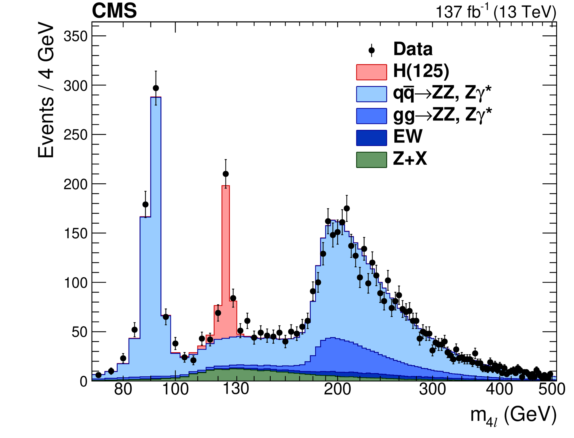
Pioneer Works is “an artist and scientist-led cultural center in Red Hook, Brooklyn that fosters innovative thinking through the visual and performing arts, technology, music, and science.” It’s a cool place: if you’re in the New York area, check them out! Among many other activities, they host a series called “Picture This,” in which scientists ruminate over scientific images that they particularly like. My own contribution to this series has just come out, in which I expound upon the importance and meaning of this graph from the CMS experimental collaboration at the Large Hadron Collider [LHC]. (The ATLAS experimental collaboration at the LHC has made essentially identical images.)

The point of the article is to emphasize the relation between the spikes seen in this graph and the images of musical frequencies that one might see in a recording studio (as in this image from this paper). The similarity is not an accident.

Each of the two biggest spikes is a sign of an elementary “particle”; the Z boson is the left-most spike, and the Higgs boson is the central spike. What is spiking is the probability of creating such a particle as a function of the energy of some sort of physical process (specifically, a collision of objects that are found inside protons), plotted along the horizontal axis. But energy E is related to the mass m of the “particle” (via E=mc2) and it is simultaneously related to the frequency f of the vibration of the “particle” (via the Planck-Einstein equation E = hf)… and so this really is a plot of frequencies, with spikes reflecting cosmic resonances analogous to the resonances of musical instruments. [If you find this interesting and would like more details, it was a major topic in my book.]

The title of the article refers to the fact that the Z boson and Higgs boson frequencies are out of tune, in the sense that if you slowed down their frequencies and turned them into sound, they’d be dissonant, and not very nice to listen to. The same goes for all the other frequencies of the elementary “particles”; they’re not at all in tune. We don’t know why, because we really have no idea where any of these frequencies come from. The Higgs field has a major role to play in this story, but so do other important aspects of the universe that remain completely mysterious. And so this image, which shows astonishingly good agreement between theoretical predictions (colored regions) and LHC data (black dots), also reveals how much we still don’t understand about the cosmos.

[An immediate continuation of Part 1, which you should definitely read first; today’s post is not stand-alone.]

The Asymmetry Between Location and Motion

We are in the middle of trying to figure out if the electron (or other similar object) could possibly be of infinitesimal size, to match the naive meaning of the words “elementary particle.” In the last post, I described how 1920’s quantum physics would envision an electron (or other object) in a state |P0> of definite momentum or a state |X0> of definite position (shown in Figs. 1 and 2 from last time.)

If it is meaningful to say that “an electron is really is an object whose diameter is zero”, we would naturally expect to be able to put it into a state in which its position is clearly defined and located at some specific point X0 — namely, we should be able to put it into the state |X0>. But do such states actually exist?

Symmetry and Asymmetry

In Part 1 we saw all sorts of symmetry between momentum and position:

• the symmetry between x and p in the Heisenberg uncertainty principle,
• the symmetry between the states |X0> and |P0>,
• the symmetry seen in their wave functions as functions of x and p shown in Figs. 1 and 2 (and see also 1a and 2a, in the side discussion, for more symmetry.)

This symmetry would seem to imply that if we could put any object, including an elementary particle, in the state |P0>, we ought to be able to put it into a state |X0>, too.

But this logic won’t follow, because in fact there’s an even more important asymmetry. The states |X0> and |P0> differ crucially. The difference lies in their energy.

Who cares about energy?

There are a couple of reasons we should care, closely related. First, just as there is a relationship between position and momentum, there is a relationship between time and energy: energy is deeply related to how wave functions evolve over time. Second, energy has its limits, and we’re going to see them violated.

Energy and How Wave Functions Change Over Time

In 1920s quantum physics, the evolution of our particle’s wave function depends on how much energy it has… or, if its energy is not definite, on the various possible energies that it may have.

Definite Momentum and Energy: Simplicity

This change with time is simple for the state |P0>, because this state, with definite momentum, also has definite energy. It therefore evolves in a very simple way: it keeps its shape, but moves with a constant speed.

Figure 5: In the state |P0>, shown in Fig. 1 of Part 1, the particle has definite momentum and energy and moves steadily at constant speed; the particle’s position is completely unknown at all times.

How much energy does it have? Well, in 1920s quantum physics, just as in pre-1900 physics, the motion-energy E of an isolated particle of definite momentum p is

• E = p2/2m

where m is the particle’s mass. Where does this formula come from? In first-year university physics, we learn that a particle’s momentum is mv and that its motion-energy is mv2/2 = (mv)2/2m = p2/2m; so in fact this is a familiar formula from centuries ago.

Less Definite Momentum and Energy: Greater Complexity

What about the compromise states mentioned in Part 1, the ones that lie somewhere between the extreme states |X0> and |P0>, in which the particle has neither definite position nor definite momentum? These “Gaussian wave packets” appeared in Fig. 3 and 4 of Part 1. The state of Fig. 3 has less definite momentum than the |P0> state, but unlike the latter, it has a rough location, albeit broadly spread out. How does it evolve?

As seen in Fig. 6, the wave still moves to the left, like the |P0> state. But this motion is now seen not only in the red and blue waves which represent the wave function itself but also in the probability for where to find the particle’s position, shown in the black curve. Our knowledge of the position is poor, but we can clearly see that the particle’s most likely position moves steadily to the left.

Figure 6: In a state with less definite momentum than |P0>, as shown in Fig. 3 of Part 1, the particle has less definite momentum and energy, but its position is roughly known, and its most likely position moves fairly steadily at near-constant speed. If we watched the wave function for a long time, it would slowly spread out.

What happens if the particle’s position is better known and the momentum is becoming quite uncertain? We saw what a wave function for such a particle looks like in Fig. 4 of Part 1, where the position is becoming quite well known, but nowhere as precisely as in the |X0> state. How does this wave function evolve over time? This is shown in Fig. 7.

Figure 7: In a state with better known position, shown in Fig. 4 of Part 1, the particle’s position is initially well known but becomes less and less certain over time, as its indefinite momentum and energy causes it to move away from its initial position at a variety of possible speeds.

We see the wave function still indicates the particle is moving to the left. But the wave function spreads out rapidly, meaning that our knowledge of its position is quickly decreasing over time. In fact, if you look at the right edge of the wave function, it has barely moved at all, so the particle might be moving slowly. But the left edge has disappeared out of view, indicating that the particle might be moving very rapidly. Thus the particle’s momentum is indeed very uncertain, and we see this in the evolution of the state.

This uncertainty in the momentum means that we have increased uncertainty in the particle’s motion-energy. If it is moving slowly, its motion-energy is low, while if it is moving rapidly, its motion-energy is much higher. If we measure its motion-energy, we might find it anywhere in between. This is why its evolution is so much more complex than that seen in Fig. 5 and even Fig. 6.

Near-Definite Position: Breakdown

What happens as we make the particle’s position better and better known, approaching the state |X0> that we want to put our electron in to see if it can really be thought of as a true particle within the methods of 1920s quantum physics?

Well, look at Fig. 8, which shows the time-evolution of a state almost as narrow as |X0> .

Figure 8: the time-evolution of a state almost as narrow as |X0>.

Now we can’t even say if the particle is going to the left or to the right! It may be moving extremely rapidly, disappearing off the edges of the image, or it may remain where it was initially, hardly moving at all. Our knowledge of its momentum is basically nil, as the uncertainty principle would lead us to expect. But there’s more. Even though our knowledge of the particle’s position is initially excellent, it rapidly degrades, and we quickly know nothing about it.

We are seeing the profound asymmetry between position and momentum:

• a particle of definite momentum can retain that momentum for a long time,
• a particle of definite position immediately becomes one whose position is completely unknown.

Worse, the particle’s speed is completely unknown, which means it can be extremely high! How high can it go? Well, the closer we make the initial wave function to that of the state |X0>, the faster the particle can potentially move away from its initial position — until it potentially does so in excess of the cosmic speed limit c (often referred to as the “speed of light”)!

That’s definitely bad. Once our particle has the possibility of reaching light speed, we need Einstein’s relativity. But the original quantum methods of Heisenberg-Born-Jordan and Schrödinger do not account for the cosmic speed limit. And so we learn: in the 1920s quantum physics taught in undergraduate university physics classes, a state of definite position simply does not exist.

Isn’t it Relatively Easy to Resolve the Problem?

But can’t we just add relativity to 1920s quantum physics, and then this problem will take care of itself?

You might think so. In 1928, Dirac found a way to combine Einstein’s relativity with Schrödinger’s wave equation for electrons. In this case, instead of the motion-energy of a particle being E = p2/2m, Dirac’s equation focuses on the total energy of the particle. Written in terms of the particle’s rest mass m [which is the type of mass that doesn’t change with speed], that total energy satisfies the equation

For stationary particles, which have p=0, this equation reduces to E=mc2, as it must.

This does indeed take care of the cosmic speed limit; our particle no longer breaks it. But there’s no cosmic momentum limit; even though v has a maximum, p does not. In Einstein’s relativity, the relation between momentum and speed isn’t p=mv anymore. Instead it is

which gives the old formula when v is much less than c, but becomes infinite as v approaches c.

Not that there’s anything wrong with that; momentum can be as large as one wants. The problem is that, as you can see for the formula for energy above, when p goes to infinity, so does E. And while that, too, is allowed, it causes a severe crisis, which I’ll get to in a moment.

Actually, we could have guessed from the start that the energy of a particle in a state of definite position |X0> would be arbitrarily large. The smaller is the position uncertainty Δx, the larger is the momentum uncertainty Δp; and once we have no idea what the particle’s momentum is, we may find that it is huge — which in turn means its energy can be huge too.

Notice the asymmetry. A particle with very small Δp must have very large Δx, but having an unknown location does not affect an isolated particle’s energy. But a particle with very small Δx must have very large Δp, which inevitably means very large energy.

The Particle(s) Crisis

So let’s try to put an isolated electron into a state |X0>, knowing that the total energy of the electron has some probability of being exceedingly high. In particular, it may be much, much larger — tens, or thousands, or trillions of times larger — than mc2 [where again m means the “rest mass” or “invariant mass” of the particle — the version of mass that does not change with speed.]

The problem that cannot be avoided first arises once the energy reaches 3mc2 . We’re trying to make a single electron at a definite location. But how can we be sure that 3mc2 worth of energy won’t be used by nature in another way? Why can’t nature use it to make not only an electron but also a second electron and a positron? [Positrons are the anti-particles of electrons.] If stationary, each of the three particles would require mc2 for its existence.

If electrons (not just the electron we’re working with, but electrons in general) didn’t ever interact with anything, and were just incredibly boring, inert objects, then we could keep this from happening. But not only would this be dull, it simply isn’t true in nature. Electrons do interact with electromagnetic fields, and with other things too. As a result, we can’t stop nature from using those interactions and Einstein’s relativity to turn 3mc2 of energy into three slow particles — two electrons and a positron — instead of one fast particle!

For the state |X0> with Δx = 0 and Δp = infinity, there’s no limit to the energy; it could be 3mc2, 11mc2, 13253mc2, 9336572361mc2. As many electron/positron pairs as we like can join our electron. The |X0> state we have ended up with isn’t at all like the one we were aiming for; it’s certainly not going to be a single particle with a definite location.

Our relativistic version of 1920s quantum physics simply cannot handle this proliferation. As I’ve emphasized, an isolated physical system has only one wave function, no matter how many particles it has, and that wave function exists in the space of possibilities. How big is that space of possibilities here?

Normally, if we have N particles moving in d dimensions of physical space, then the space of possibilities has N-times-d dimensions. (In examples that I’ve given in this post and this one, I had two particles moving in one dimension, so the space of possibilities was 2×1=2 dimensional.) But here, N isn’t fixed. Our state |X0> might have one particle, three, seventy one, nine thousand and thirteen, and so on. And if these particles are moving in our familiar three dimensions of physical space, then the space of possibilities is 3 dimensional if there is one particle, 9 dimensional if there are three particles, 213 dimensional if there are seventy-one particles — or said better, since all of these values of N are possible, our wave function has to simultaneously exist in all of these dimensional spaces at the same time, and tell us the probability of being in one of these spaces compared to the others.

Still worse, we have neglected the fact that electrons can emit photons — particles of light. Many of them are easily emitted. So on top of everything else, we need to include arbitrary numbers of photons in our |X0> state as well.

Good Heavens. Everything is completely out of control.

How Small Can An Electron Be (In 1920s Quantum Physics?)

How small are we actually able to make an electron’s wave function before the language of the 1920s completely falls apart? Well, for the wave function describing the electron to make sense,

• its motion-energy must be below mc2, which means that
• p has to be small compared to mc , which means that
• Δp has to be small compared to mc , which means that
• by Heisenberg’s uncertainty principle, Δx has to be large compared to h/(4πmc)

This distance (up to the factor of 1/4π) is known as a particle’s Compton wavelength, and it is about 10-13 meters for an electron. That’s about 1/1000 of the distance across an atom, but 100 times the diameter of a small atomic nucleus. Therefore, 1920s quantum physics can describe electrons whose wave functions allow them to range across atoms, but cannot describe an electron restricted to a region the size of an atomic nucleus, or of a proton or neutron, whose size is 10-15 meters. It certainly can’t handle an electron restricted to a point!

Let me reiterate: an electron cannot be restricted to a region the size of a proton and still be described by “quantum mechanics”.

As for neutrinos, it’s much worse; since their masses are much smaller, they can’t even be described in regions whose diameter is that of a thousand atoms!

The Solution: Relativistic Quantum Field Theory

It took scientists two decades (arguably more) to figure out how to get around this problem. But with benefit of hindsight, we can say that it’s time for us to give up on the quantum physics of the 1920s, and its image of an electron as a dot — as an infinitesimally small object. It just doesn’t work.

Instead, we now turn to relativistic quantum field theory, which can indeed handle all this complexity. It does so by no longer viewing particles as fundamental objects with infinitesimal size, position x and momentum p, and instead seeing them as ripples in fields. A quantum field can have any number of ripples — i.e. as many particles and anti-particles as you want, and more generally an indefinite number. Along the way, quantum field theory explains why every electron is exactly the same as every other. There is no longer symmetry between x and p, no reason to worry about why states of definite momentum exist and those of definite position do not, and no reason to imagine that “particles” [which I personally think are more reasonably called “wavicles“, since they behave much more like waves than particles] have a definite, unchanging shape.

The space of possibilities is now the space of possible shapes for the field, which always has an infinite number of dimensions — and indeed the wave function of a field (or of multiple fields) is a function of an infinite number of variables (really a function of a function [or of multiple functions], called a “functional”).

Don’t get me wrong; quantum field theory doesn’t do all this in a simple way. As physicists tried to cope with the difficult math of quantum field theory, they faced many serious challenges, including apparent infinities everywhere and lots of consistency requirements that needed to be understood. Nevertheless, over the past seven decades, they solved the vast majority of these problems. As they did so, field theory turned out to agree so well with data that it has become the universal modern language for describing the bricks and mortar of the universe.

Yet this is not the end of the story. Even within quantum field theory, we can still find ways to define what we mean by the “size” of a particle, though doing so requires a new approach. Armed with this definition, we do now have clear evidence that electrons are much smaller than protons. And so we can ask again: can an elementary “particle” [wavicle] have zero size?

We’ll return to this question in later posts.

This is admittedly a provocative title coming from a particle physicist, and you might think it tongue-in-cheek. But it’s really not.

We live in a cosmos with quantum physics, relativity, gravity, and a bunch of elementary fields, whose ripples we call elementary particles. These elementary “particles” include objects like electrons, photons, quarks, Higgs bosons, etc. Now if, in ordinary conversation in English, we heard the words “elementary” and “particle” used together, we would probably first imagine that elementary particles are tiny balls, shrunk down to infinitesimal size, making them indivisible and thus elementary — i.e., they’re not made from anything smaller because they’re as small as could be. As mere points, they would be objects whose diameter is zero.

But that’s not what they are. They can’t be.

I’ll tell this story in stages. In my last post, I emphasized that after the Newtonian view of the world was overthrown in the early 1900s, there emerged the quantum physics of the 1920s, which did a very good job of explaining atomic physics and a variety of other phenomena. In atomic physics, the electron is indeed viewed as a particle, though with behavior that is quite unfamiliar. The particle no longer travels on a path through physical space, and instead its behavior — where it is, and where it is going — is described probabilistically, using a wave function that exists in the space of possibilities.

But as soon became clear, 1920s quantum physics forbids the very existence of elementary particles.

In 1920s Quantum Physics, True Particles Do Not Exist

To claim that particles do not exist in 1920s quantum physics might seem, at first, absurd, especially to people who took a class on the subject. Indeed, in my own blog post from last week, I said, without any disclaimers, that “1920s quantum physics treats an electron as a particle with position x and momentum p that are never simultaneously definite.” (Recall that momentum is about motion; in pre-quantum physics, the momentum of an object is its mass m times its speed v.) Unless I was lying to you, my statement would seem to imply that the electron is allowed to have definite position x if its momentum p is indefinite, and vice versa. And indeed, that’s what 1920s quantum physics would imply.

To see why this is only half true, we’re going to examine two different perspectives on how 1920s quantum physics views location and motion — position x and momentum p.

1. There is a perfect symmetry between position and momentum (today’s post)
2. There is a profound asymmetry between position and momentum (next post)

Despite all the symmetry, the asymmetry turns out to be essential, and we’ll see (in the next post) that it implies particles of definite momentum can exist, but particles of definite position cannot… not in 1920s quantum physics, anyway.

The Symmetry Between Location and Motion

The idea of a symmetry between location and motion may seem pretty weird at first. After all, isn’t motion the change in something’s location? Obviously the reverse is not generally true: location is not the change in something’s motion! Instead, the change in an object’s motion is called its “acceleration” (a physics word that includes what in English we’d call acceleration, deceleration and turning.) In what sense are location and motion partners?

The Uncertainty Principle of Werner Heisenberg

In a 19th century reformulation of Newton’s laws of motion that was introduced by William Rowan Hamilton — keeping the same predictions, but rewriting the math in a new way — there is a fundamental symmetry between position x and momentum p. This way of looking at things is carried on into quantum physics, where we find it expressed most succinctly through Heisenberg’s uncertainty principle, which specifically tells us that we cannot know a object’s position and momentum simultaneously.

This might sound vague, but Heisenberg made his principle very precise. Let’s express our uncertainty in the object’s position as Δx. (Heisenberg defined this as the average value of x2 minus the squared average value of x. Less technically, it means that if we think the particle is probably at a position x0, an uncertainty of Δx means that the particle has a 95% chance of being found anywhere between x0-2Δx and x0+2Δx.) Let’s similarly express our uncertainty about the object’s momentum (which, again, is naively its speed times its mass) as Δp. Then in 1920s quantum physics, it is always true that

• Δp Δx > h / (4π)

where h is Planck’s constant, the mascot of all things quantum. In other words, if we know our uncertainty on an object’s position Δx, then the uncertainty on its momentum cannot be smaller than a minimum amount:

• Δp > h / (4π Δx) .

Thus, the better we know an object’s position, implying a smaller Δx, the less we can know about the object’s momentum — and vice versa.

This can be taken to extremes:,

• if we knew an object’s motion perfectly — if Δp is zero — then Δx = h / (4π Δp) = infinity, in which case we have no idea where the particle might be
• if we knew an object’s location perfectly — if Δx is zero — then Δp = h / (4π Δx) = infinity, in which case we have no idea where or how fast the particle might be going.

You see everything is perfectly symmetric: the more I know about the object’s location, the less I can know about its motion, and vice versa.

(Note: My knowledge can always be worse. If I’ve done a sloppy measurement, I could be very uncertain about the object’s location and very uncertain about its location. The uncertainty principle contains a greater-than sign (>), not an equals sign. But I can never be very certain about both at the same time.)

An Object with Known Motion

What does it mean for an object to have zero uncertainty in its position or its motion? Quantum physics of the 1920s asserts that any system is described by a wave function that tells us the probability for where we might find it and what it might be doing. So let’s ask: what form must a wave function take to describe a single particle with perfectly known momentum p?

The physical state corresponding to a single particle with perfectly known momentum P0 , which is often denoted |P0>, has a wave function

times an overall constant which we don’t have to care about. Notice the ; this is a complex number at each position x. I’ve plotted the real and imaginary parts of this function in Fig. 1 below. As you see, both the real (red) and imaginary (blue) parts look like a simple wave, of infinite extent and of constant wavelength and height.

Figure 1: In red and blue, the real and imaginary parts of the wave function describing a particle of known momentum (up to an overall constant). In black is the square of the wave function, showing that the particle has equal probability to be at each possible location.

Now, what do we learn from the wave function about where this object is located? The probability for finding the object at a particular position X is given by the absolute value of the wave function squared. Recall that if I have any complex number z = x + i y, then its absolute value squared |z2| equals |x2|+|y2|. Therefore the probability to be at X is proportional to

(again multiplied by an overall constant.) Notice, as shown by the black line in Fig. 1, this is the same no matter what X is, which means the object has an equal probability to be at any location we choose. And so, we have absolutely no idea of where it is; as far as we’re concerned, its position is completely random.

An Object with Known Location

As symmetry requires, we can do the same for a single object with perfectly known position X0. The corresponding physical state, denoted |X0>, has a wave function

again times an overall constant. Physicists call this a “delta function”, but it’s just an infinitely narrow spike of some sort. I’ve plotted something like it in Figure 2, but you should imagine it being infinitely thin and infinitely high, which obviously I can’t actually draw.

This wave function tells us that the probability that the object is at any point other than X0 is equal to zero. You might think the probability of it being at X0 is infinity squared, but the math is clever and the probability that it is at X0 is exactly 1. So if the particle is in the physical state |X0>, we know exactly where it is: it’s at position X0.

Figure 2: The wave function describing a particle of known position (up to an overall constant). The square of the wave function is in black, showing that the particle has zero probability to be anywhere except at the spike. The real and imaginary parts (in red and blue) are mostly covered by the black line.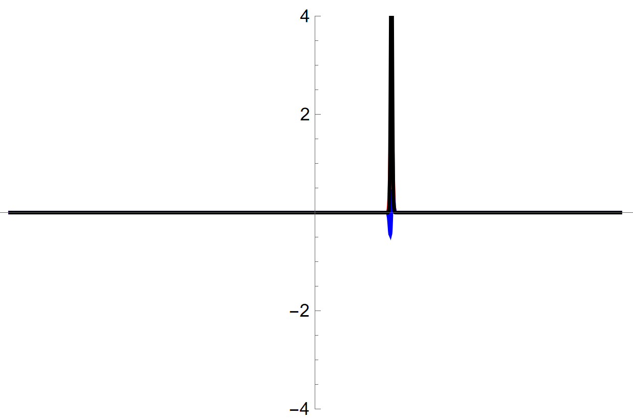

What do we know about its motion? Well, we saw in Fig. 1 that to know an object’s momentum perfectly, its wave function should be a spread-out, simple wave with a constant wavelength. This giant spike, however, is as different from nice simple waves as it could possibly be. So |X0> is a state in which the momentum of the particle, and thus its motion, is completely unknown. [To prove this vague argument using math, we would use a Fourier transform; we’ll get more insight into this in a later post.]

So we have two functions, as different from each other as they could possibly be,

• Fig. 1 describing an object with a definite momentum and completely unknown position, and
• Fig. 2 describing an object with definite position and completely unknown momentum.

CAUTION: We might be tempted to think: “oh, Fig. 1 is the wave, and Fig. 2 is the particle”. Indeed the pictures make this very tempting! But no. In both cases, we are looking at the shape of a wave function that describes where an object, perhaps a particle, is located. When people talk about an electron being both wave and particle, they’re not simply referring to the relation between momentum states and position states; there’s more to it than that.

CAUTION 2: Do not identify the wave function with the particle it describes!!! It is not true that each particle has its own wave function. Instead, if there were two particles, there would still be only one wave function, describing the pair of particles. See this post and this one for more discussion of this crucial point.

Objects with More or Less Uncertainty

We can gain some additional intuition for this by stepping back from our extreme |P0> and |X0> states, and looking instead at compromise states that lie somewhere between the extremes. In these states, neither p nor x is precisely known, but the uncertainty of one is as small as it can be given the uncertainty of the other. These special states are often called “Gaussian wave packets”, and they are ideal for showing us how Heisenberg’s uncertainty principle plays out.

In Fig. 3 I’ve shown a wave function for a particle whose position is poorly known but whose momentum is better known. This wave function looks like a trimmed version of the |P0> state of Fig. 1, and indeed the momentum of the particle won’t be too far from P0. The position is clearly centered to the right of the vertical axis, but it has a large probability to be on the left side, too. So in this state, Δp is small and Δx is large.

Figure 3: A wave function similar to that of Fig. 1, describing a particle that has an almost definite momentum and a rather uncertain position.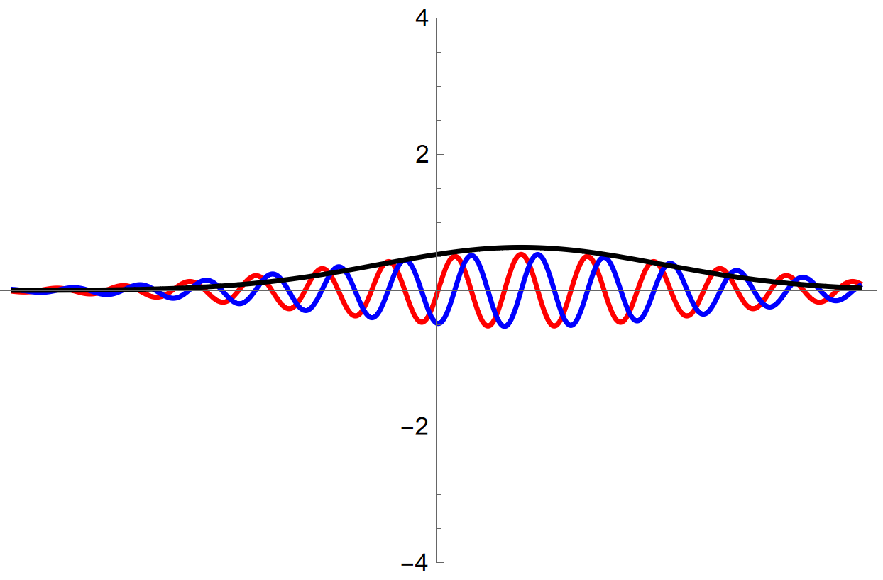

In Fig. 4 I’ve shown a wave function of a wave packet that has the situation reversed: its position is well known and its momentum is not. It looks like a smeared out version of the |X0> state in Fig. 2, and so the particle is most likely located quite close to X0. We can see the wave function shows some wavelike behavior, however, indicating the particle’s momentum isn’t completely unknown; nevertheless, it differs greatly from the simple wave in Fig. 1, so the momentum is pretty uncertain. So here, Δx is small and Δp is large.

Figure 4: A wave function similar to that of Fig. 2, describing a particle that has an almost definite position and a highly uncertain momentum.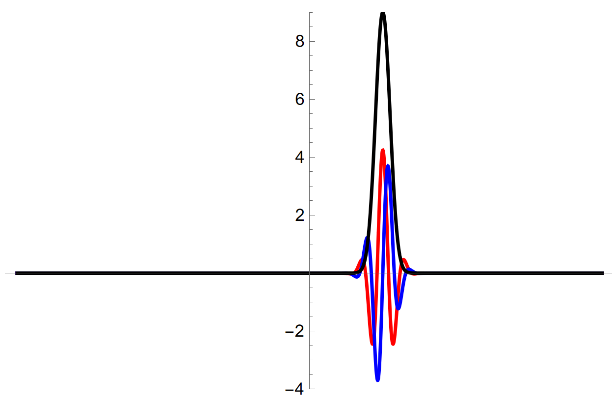

In this way we can interpolate however we like between Figs. 1 and 2, getting whatever uncertainty we want on momentum and position as long as they are consistent with Heisenberg’s uncertainty relation.

Wave functions in the space of possible momenta There’s even another more profound, but somewhat more technical, way to see the symmetry in action; click here if you are interested.

As I’ve emphasized recently (and less recently), the wave function of a system exists in the space of possibilities for that system. So far I’ve been expressing this particle’s wave function as a space of possibilities for the particle’s location — in other words, I’ve been writing it, and depicting it in Figs. 1 and 2, as Ψ(x). Doing so makes it more obvious what the probabilities are for where the particle might be located, but to understand what this function means for what the particle’s motion takes some reasoning.

But I could instead (thanks to the symmetry between position and momentum) write the wave function in the space of possibilities for the particle’s motion! In other words, I can take the state |P0>, in which the particle has definite momentum, and write it either as Ψ(x), shown in Fig. 1, or as Ψ(p), shown in Fig. 1a.

Figure 1a: The wave function of Fig. 1, written in the space of possibilities of momenta instead of the space of possibilities of position; i.e., the horizontal axis show the particle’s momentum p, not its position x as is the case in Figs. 1 and 2. This shows the particle’s momentum is definitely known. Compare this with Fig. 2, showing a different wave function in which the particle’s position is definitely known.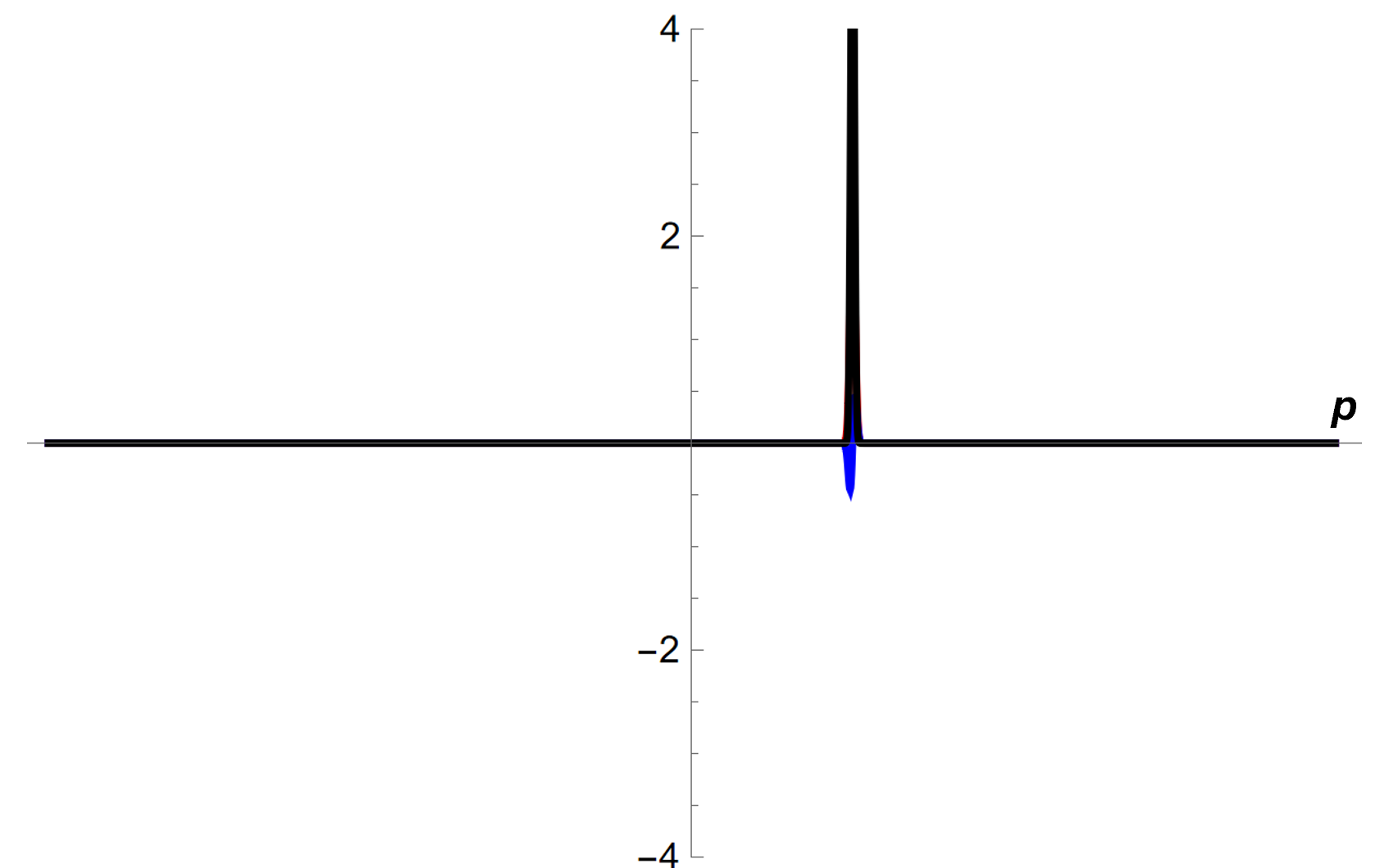

Remarkably, Fig. 1a looks just like Fig. 2 — except for one crucial thing. In Fig. 2, the horizontal axis is the particle’s position. In Fig. 1a, however, the horizontal axis is the particle’s momentum — and so while Fig. 2 shows a wave function for a particle with definite position, Fig. 1a shows a wave function for a particle with definite momentum, the same wave function as in Fig. 1.

We can similarly write the wave function of Fig. 2 in the space of possibilities for the particle’s position, and not surprisingly, the resulting Fig. 2a looks just like Fig. 1, except that its horizontal axis represents p, and so in this case we have no idea what the particle’s momentum is — neither the particle’s speed nor its direction.

Fig. 2a: As in Fig. 1a, the wave function in Fig. 2 written in terms of the particle’s momentum p.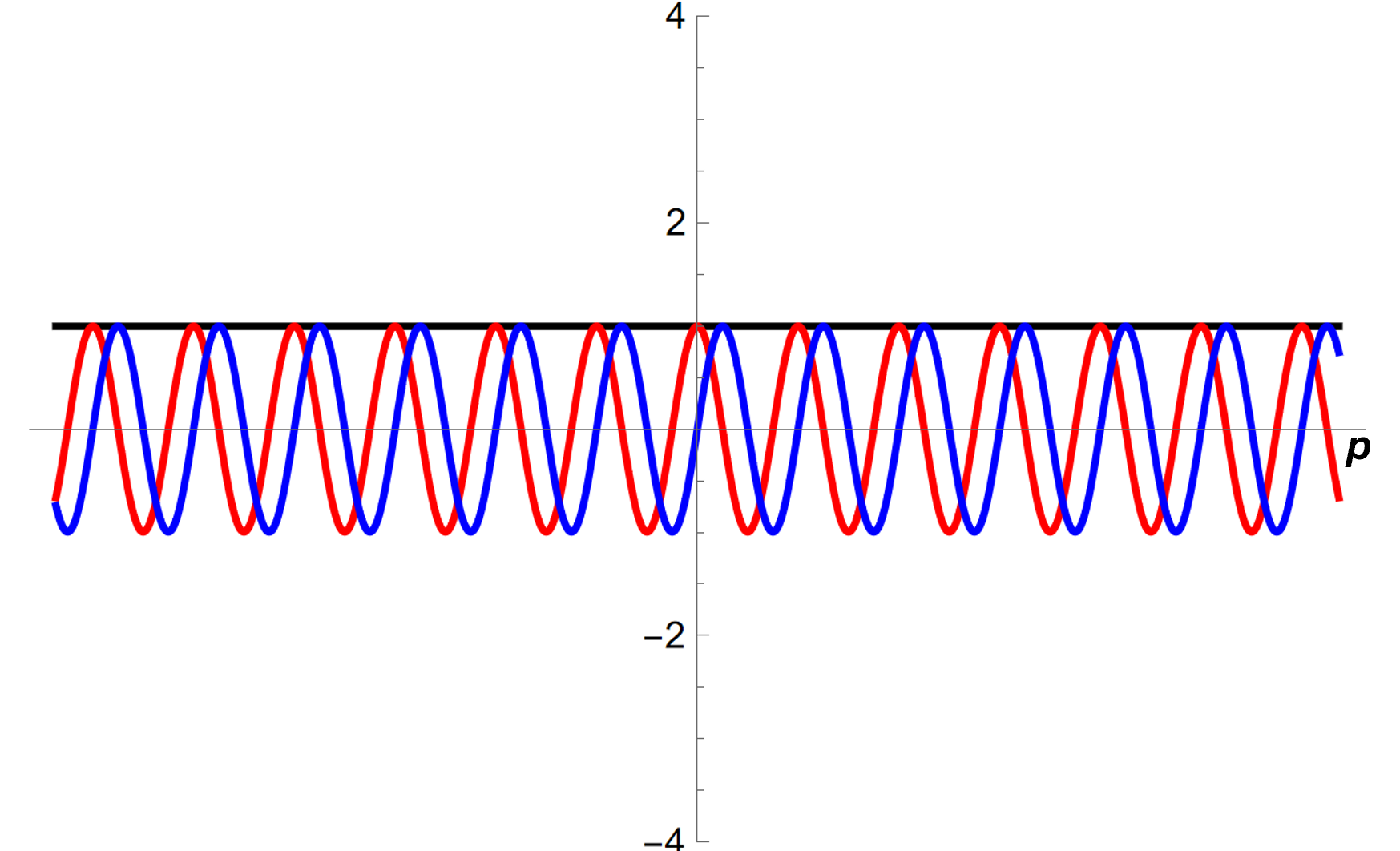

The relationship between Fig. 1 and Fig. 1a is that each is the Fourier transform of the other [where the momentum is related to the inverse wavelength of the wave obtained in the transform.] Similarly, Figs. 2 and 2a are each other’s Fourier transforms.

In short, the wave function for the state |P0> (as a function of position) in Fig. 1 looks just like the wave function for the state |X0> (as a function of momentum) in Fig. 2a, and a similar relation holds for Figs. 2 and 1a. Everything is symmetric!

The Symmetry and the Particle…

So, what’s this all got to do with electrons and other elementary particles? Well, if a “particle” is really and truly a particle, an object of infinitesimal size, then we certainly ought to be able to put it, or at least imagine it, in a position state like |X0>, in which its position is clearly X0 with no uncertainty. Otherwise how could we ever even tell if its size is infinitesimal? (This is admittedly a bit glib, but the rough edges to this argument won’t matter in the end.)

That’s where this symmetry inherent in 1920s quantum physics comes in. We do in fact see states of near-definite momentum — of near-definite motion. We can create them pretty easily, for instance in narrow electron beams, where the electrons have been steered by electric and magnetic fields so they have very precisely defined momentum. Making position states is trickier, but it would seem they must exist, thanks to the symmetry of momentum and position.

But they don’t. And that’s thanks to a crucial asymmetry between location and motion that we’ll explore next time.

As expected, the Musk/Trump administration has aimed its guns at the US university system, deciding that universities that get grants from the federal government’s National Institute of Health will have their “overhead” capped at 15%. Overhead is the money that is used to pay for the unsung things that make scientific research at universities and medical schools possible. It pays for staff that keep the university running — administrators and accountants in business offices, machinists who help build experiments, janitorial staff, and so on — as well as the costs for things like building maintenance and development, laboratory support, electricity and heating, computing clusters, and the like.

I have no doubt that the National Science Foundation, NASA, and other scientific funding agencies will soon follow suit.

As special government employee Elon Musk wrote on X this weekend, “Can you believe that universities with tens of billions in endowments were siphoning off 60% of research award money for ‘overhead’? What a ripoff!”

The actual number is 38%. Overhead of 60% is measured against the research part of the award, not the total award, and so the calculation is 60%/(100%+60%) = 37.5%, not 60%/100%=60%. This math error is a little worrying, since the entire national budget is under Musk’s personal control. And never mind that a good chunk of that money often comes back to research indirectly, or that “siphon”, a loaded word implying deceit, is inappropriate — the overhead rate for each university isn’t a secret.

Is overhead at some universities too high? A lot of scientific researchers feel that it is. One could reasonably require a significant but gradual reduction of the overhead rate over several years, which would cause limited damage to the nation’s research program. But dropping the rate to 15%, and doing so over a weekend, will simply crush budgets at every major academic research institution in the country, leaving every single one with a significant deficit. Here is one estimate of the impact on some of the United States leading universities; I can’t quickly verify these details myself, but the numbers look to be at the right scale. They are small by Musk standards, but they come to something very roughly like $10000, more or less, per student, per year.

Also, once the overhead rate is too low, having faculty doing scientific research actually costs a university money. Every new grant won by a scientist at the university makes the school’s budget deficit worse. Once that line is crossed, a university may have to limit research… possibly telling some fraction of its professors not to apply for grants and to stop doing research.

It is very sad that Mr. Musk considers the world’s finest medical/scientific research program, many decades in the making and of such enormous value to the nation, to be deserving of this level of disruption. While is difficult to ruin our world-leading medical and scientific research powerhouse overnight, this decision (along with the funding freeze/not-freeze/kinda-freeze from two weeks ago) is a good start. Even if this cut is partially reversed, the consequences on health care and medicine in this country, and on science and engineering more widely, will be significant and long-lasting — because if you were one of the world’s best young medical or scientific researchers, someone who easily could get a job in any country around the globe, would you want to work in the US right now? The threat of irrational chaos that could upend your career at any moment is hardly appealing.